Download

1 / 189
1.92k likes | 2.08k Vues
Advanced Topics in Computer Systems: Machine Learning and Data Mining Systems Winter 2007. Stan Matwin Professor School of Information Technology and Engineering/ École d’ingénierie et de technologie de l’information University of Ottawa Canada. Goals of this course.

E N D
Advanced Topics in Computer Systems: Machine Learning and Data Mining SystemsWinter 2007 Stan Matwin Professor School of Information Technology and Engineering/ École d’ingénierie et de technologie de l’information University of Ottawa Canada
Goals of this course • Dual seminar/tutorial structure • The tutorial part will teach basic concepts of Machine Learning (ML) and Data Mining (DM) • The seminar part will • introduce interesting areas of current and future research • Introduce successful applications • Preparation to enable advanced self-study on ML/DM
Course outline • Machine Learning/Data Mining: basic terminology. • Symbolic learning: Decision Trees; • Basic Performance Evaluation • Introduction to the WEKA system • Probabilistic learning: Bayesian learning. • Text classification
Kernel-based methods: Support Vector Machines • Ensemble-based methods: boosting • Advanced Performance Evaluation: ROC curves • Applications in bioinformatics • Data mining concepts and techniques: Association Rules • Feature selection and discretization
Machine Learning / Data Mining: basic terminology • Machine Learning: • given a certain task, and a data set that constitutes the task, • ML provides algorithms that resolve the task based on the data, and the solution improves with time • Examples: • predicting lottery numbers next Saturday • detecting oil spills on sea surface • assigning documents to a folder • identifying people likely to want a new credit card (cross selling)
Data Mining: extracting regularities from a VERY LARGE dataset/database as part of a business/application cycle • examples: • cell phone fraud detection • customer churn • direct mail targeting/ cross sell • prediction of aircraft component failures
Basic ML tasks • Supervised learning • classification/concept learning • estimation: essentially, extrapolation • Unsupervised learning: • clustering: finding groups of “similar” objects • associations: in a database, finding that some values of attributes go with some other
Concept learning (also known asclassification): a definition • the concept learning problem: • given • a set E = {e1, e2, …, en} of training instances of concepts, each labeled with the name of a concept C1, …,Ck to which it belongs • determine • definitions of each of C1, …,Ck which correctly cover E. Each definition is a concept description
Dimensions of concept learning • representation; • data • symbolic • numeric • concept description • attribute-value (propositional logic) • relational (first order logic) • Language of examples and hypotheses • Attribute-value (AV) = propositional representation • Relational (ILP) = first-order logic representation • method of learning • top-down • bottom-up (covering) • different search algorithms
2. Decision Trees wage incr. 1st yr A decision tree as a concept representation: working hrs statutory holidays good good contribution to hlth plan wage incr. 1st yr bad bad good bad good
building a univariate (single attribute is tested) decision tree from a set T of training cases for a concept C with classes C1,…Ck • Consider three possibilities: • T contains 1 or more cases all belonging to the same class Cj. The decision tree for T is a leaf identifying class Cj • T contains no cases. The tree is a leaf, but the label is assigned heuristically, e.g. the majority class in the parent of this node
T contains cases from different classes. T is divided into subsets that seem to lead towards collections of cases. A test t based on a single attribute is chosen, and it partitions T into subsets {T1,…,Tn}. The decision tree consists of a decision node identifying the tested attribute, and one branch for ea. outcome of the test. Then, the same process is applied recursively to ea.Ti
Choosing the test • why not explore all possible trees and choose the simplest (Occam’s razor)? But this is an NP complete problem. E.g. in the ‘union’ example there are millions of trees consistent with the data • notation: S: set of the training examples; freq(Ci, S) = number of examples in S that belong to Ci; • information measure (in bits) of a message is - log2 of the probability of that message • idea: to maximize the difference between the info needed to identify a class of an example in T, and the the same info after T has been partitioned in accord. with a test X
selecting 1 case and announcing its class has info meas. - log2(freq(Ci, S)/|S|) bits to find information pertaining to class membership in all classes: info(S) = -(freq(Ci, S)/|S|)*log2(freq(Ci, S)/|S|) after partitioning according to outcome of test X: infoX(T) = |Ti|/|T|*info(Ti) gain(X) = info(T) - infoX(T) measures the gain from partitioning T according to X We select X to maximize this gain
Data for learning the weather (play/don’t play) concept (Witten p. 10) Info(S) = 0.940
Selecting the attribute • Gain(S, Outlook) = 0.246 • Gain(S, Humidity) = 0.151 • Gain(S, Wind) = 0.048 • Gain(S, Temp) = 0.029 • Choose Outlook as the top test
Gain ratio • info gain favours tests with many outcomes (patient id example) • consider split info(X) = |Ti|/|T|*log(|Ti|/|T|) measures potential info. generated by dividing T into n classes (without considering the class info) gain ratio(X) = gain(X)/split info(X) shows the proportion of info generated by the split that is useful for classification: in the example (Witten p. 96), log(k)/log(n) maximize gain ratio
In fact, learning DTs with the gain ratio heuristic is a search:
continuous attrs • a simple trick: sort examples on the values of the attribute considered; choose the midpoint between ea two consecutive values. For m values, there are m-1 possible splits, but they can be examined linearly • cost?
From trees to rules: traversing a decision tree from root to leaf gives a rule, with the path conditions as the antecedent and the leaf as the class rules can then be simplified by removing conditions that do not contribute to discriminate the nominated class from other classes rulesets for a whole class are simplified by removing rules that do not contribute to the accuracy of the whole set
Geometric interpretation of decision trees: axis-parallel area b > b1 a1 n y a > a1 a2 a < a2 b1
Decision rules can be obtained from decision trees (1)if b>b1 then class is - (2)if b <= b1 and a > a1 then class is + (3)if b <= b1 a < a2 then class is + (4)if b <= b1 and a2 <= a <= a1 then class is - b > b1 n y a > a1 (1) (2) a < a2 notice the inference involved in rule (3) (3) (4)
lots of datasets can be obtained from ftp ics.uci.edu cd pub/machine-learning-databases contents are described in the file README in the dir machine-learning-databases at Irvine
Empirical evaluation of accuracy in classification tasks • the usual approach: • partition the set E of all labeled examples (examples with their classification labels) into a training set and a testing set • use the training set for learning, obtain a hypothesis H, set acc := 0 • for ea. element t of the testing set, apply H on t; if H(t) = label(t) then acc := acc+1 • acc := acc/|testing set|
Testing - cont’d • Given a dataset, how do we split it between the training set and the test set? • cross-validation (n-fold) • partition E into n groups • choose n-1 groups from n, perform learning on their union • repeat the choice n times • average the n results • usually, n = 3, 5, 10 • another approach - learn on all but one example, test that example. “Leave One Out”
Confusion matrix classifier-determined classifier-determined positive label negative label true positive a b label true negative c d label Accuracy = (a+d)/(a+b+c+d) a = true positives b =false negatives c = false positives d = true negatives
Precision = a/(a+c) • Recall = a/(a+b) • F-measure combines Recall and Precision: • Fb = (b2+1)*P*R / (b2 P + R) • Refelects importance of Recall versus Precision; eg F0 = P
Cost matrix • Is like confusion matrix, except costs of errors are assigned to the elements outside the diagonal (mis-classifications) • this may be important in applications, e.g. when the classifier is a diagnosis rule • see http://ai.iit.nrc.ca/bibliographies/cost-sensitive.html for a survey of learning with misclassification costs
Bayesian learning • incremental, noise-resistant method • can combine prior Knowledge (the K is probabilistic) • predictions are probabilistic
Bayes’ law of conditional probability: results in a simple “learning rule”: choose the most likely (Maximum APosteriori)hypothesis Example: Two hypo: (1) the patient has cancer (2) the patient is healthy
P(cancer) = .008 P( + |cancer) = .98 P(+|not cancer) = .03 P(not cancer) = .992 P( - |cancer) = .02 P(-|not cancer) = .97 Priors: 0.8% of the population has cancer; We observe a new patient with a positive test. How should they be diagnosed? P(cancer|+) = P(+|cancer)P(cancer) = .98*.008 = .0078 P(not cancer|+) = P(+|not cancer)P(not cancer) = .03*.992=.0298
Minimum Description Length revisiting the def. of hMAP: we can rewrite it as: or But the first log is the cost of coding the data given the theory, and the second - the cost of coding the theory
Observe that: for data, we only need to code the exceptions; the others are correctly predicted by the theory MAP principles tells us to choose the theory which encodes the data in the shortest manner the MDL states the trade-off between the complexity of the hypo. and the number of errors
Bayes optimal classifier • so far, we were looking at the “most probable hypothesis, given a priori probabilities”. But we really want the most probable classification • this we can get by combining the predictions of all hypotheses, weighted by their posterior probabilities: • this is the bayes optimal classifier BOC: Example of hypotheses h1, h2, h3 with posterior probabilities .4, .3. .3 A new instance is classif. pos. by h1 and neg. by h2, h3
Bayes optimal classifier V = {+, -} P(h1|D) = .4, P(-|h1) = 0, P(+|h1) = 1 … Classification is ” –” (show details!)
Captures probability dependencies • ea node has probability distribution: the task is to determine the join probability on the data • In an appl. a model is designed manually and forms of probability distr. Are given • Training set is used to fut the model to the data • Then probabil. Inference can be carried out, eg for prediction First five variables are observed, and the model is Used to predict diabetes P(A, N, M, I, G, D)=P(A)*P(n)*P(M|A, n)*P(D|M, A, N)*P(I|D)*P(G|I,D)
how do we specify prob. distributions? • discretize variables and represent probability distributions as a table • Can be approximated from frequencies, eg table P(M|A, N) requires 24parameters • For prediction, we want (D|A, n, M, I, G): we need a large table to do that
no other classifier using the same hypo. spac e and prior K can outperform BOC • the BOC has mostly a theoretical interest; practically, we will not have the required probabilities • another approach, Naive Bayes Classifier (NBC) under a simplifying assumption of independence of the attribute values given the class value: To estimate this, we need (#of possible values)*(#of possible instances) examples
in NBC, the conditional probabilities are estimated from training data simply as normalized frequencies: how many times a given attribute value is associated with a given class • no search! • example • m-estimate
Example (see the Dec. Tree sec. in these notes): we are trying to predict yes or no for Outlook=sunny, Temperature=cool, Humidity=high, Wind=strong P(yes)=9/14 P(no)=5/14 P(Wind=strong|yes)=3/9 P(Wind=strong|no)=3/5 etc. P(yes)P(sunny|yes)P(cool|yes)P(high|yes)Pstrong|yes)=.0053 P(yes)P(sunny|no)P(cool|no)P(high|no)Pstrong|no)=.0206 so we will predict no compare to 1R!
Further, we can not only have a decision, but also the prob. of that decision: • we rely on for the conditional probability • if the conditional probability is very small, and n is small too, then we should assume that nc is 0. But this biases too strongly the NBC. • So: smoothen; see textbook p. 85 • Instead, we will use the estimate where p is the prior estimate of probability, m is equivalent sample size. If we do not know otherwise, p=1/k for k values of the attribute; m has the effect of augmenting the number of samples of class ; large value of m means that priors p are important wrt training data when probability estimates are computed, small – less important
Text Categorization • Representations of text are very high dimensional (one feature for each word). • High-bias algorithms that prevent overfitting in high-dimensional space are best. • For most text categorization tasks, there are many irrelevant and many relevant features. • Methods that sum evidence from many or all features (e.g. naïve Bayes, KNN, neural-net) tend to work better than ones that try to isolate just a few relevant features (decision-tree or rule induction).
Naïve Bayes for Text • Modeled as generating a bag of words for a document in a given category by repeatedly sampling with replacement from a vocabulary V = {w1, w2,…wm} based on the probabilities P(wj| ci). • Smooth probability estimates with Laplace m-estimates assuming a uniform distribution over all words (p = 1/|V|) and m = |V| • Equivalent to a virtual sample of seeing each word in each category exactly once.
Text Naïve Bayes Algorithm(Train) Let V be the vocabulary of all words in the documents in D For each category ci C Let Dibe the subset of documents in D in category ci P(ci) = |Di| / |D| Let Ti be the concatenation of all the documents in Di Let ni be the total number of word occurrences in Ti For each word wj V Let nij be the number of occurrences of wj in Ti Let P(wi| ci) = (nij + 1) / (ni + |V|)