Genetic Algorithms and Ant Colony Optimisation

1. Genetic Algorithms and Ant Colony Optimisation

2. Introduction: Optimisation • Optimisation : find an extremum • Extrema can be local / global • In Rn (real numbers): methods with and without gradients • Local : • With derivative (ok : space = Rn)  gradient (possibly: first degree or even more) • Without derivative : select a point, explore the neighborood, take the best, do it again. (type hill climber, local search) • Global : • = local with different initial conditions. • Method without derivatives  GA

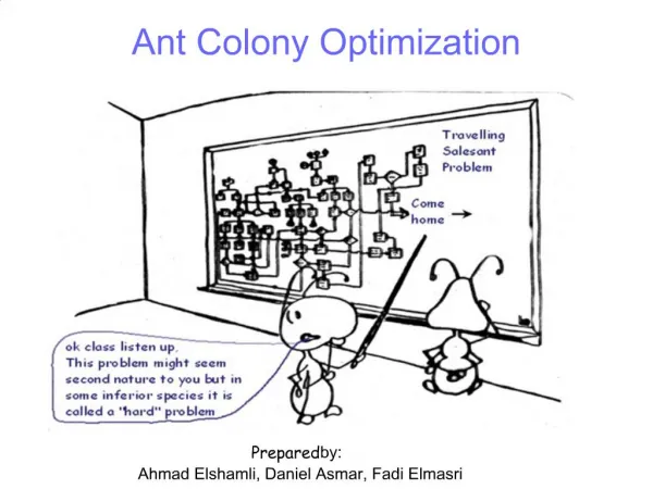
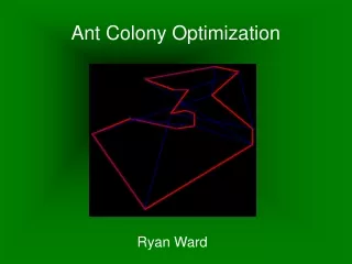
3. Combinatorial optimisation problems. • Deterministic algorithms : Explore too much and take too much time  meta-heuristiques : find rapidly a satisfactory solution • Example : Scheduling problem, packing or ordering problems • The classics of the classics : TSP • The travelling salesman problem • N cities • Find the shortest path going through each city only once • Benchmarking problems • Problems NP-complete (the time to find grows exponentially with the size of the problem (N! ~ N^(N+1/2)))

4. Genetic Algorithms: Introduction • Evolutionary computing • 1975 : John Holland  Genetic algorithms • 1992 : John Koza  Genetic programming

5. Genetic algorithms • Darwinian inspiration • Evolution = optimisation:

6. Reproduction • 2 genetic operators: • Cross-over (recombination) • Mutation • Fitness

7. The standard algorithm • Generate random population • Repeat • Evaluate fitness f(x) for each individual of the population • Create a new population (to repeat until a stopping critetion) • Selection (according to fitness) • Crossover (according to probability of crossover) • Mutation (according to probability of mutation) • evaluate the new individuals in the population (replacement) • Replace the old population by the new (better) ones • Until stop condition; return the best solution of the current population

10. Chromosones encoding • Can be influenced by the problem to solve • Examples: • Binary encoding • Permutation encoding (ordening problems) e.g. TSP problem) • Real value encoding (evolutionary strategies) • Tree encoding (genetic programming)

11. Binary Encoding Chromosome A 101100101100101011100101 Chromosome B 111111100000110000011111 • Binary encoding is the most common, mainly because first works about GA used this type of encoding.In binary encoding everychromosome is a string of bits, 0 or 1. • Example of Problem: Knapsack problem
The problem: There are things with given value and size. The knapsack has given capacity. Select things to maximize the value of things in knapsack, but do not extend knapsack capacity.
Encoding: Each bit says, if the corresponding thing is in knapsack.


12. Permutation Encoding Chromosome A 1 5 3 2 6 4 7 9 8 Chromosome B 8 5 6 7 2 3 1 4 9 • In permutation encoding, every chromosome is a string of numbers, which represents number in a sequence. • Example of Problem: Traveling salesman problem (TSP)
The problem: There are cities and given distances between them.Travelling salesman has to visit all of them, but he does not to travel very much. Find a sequence of cities to minimize travelled distance. Encoding: Chromosome says order of cities, in which salesman will visit them.

13. Value Encoding Chromosome A 1.2324 5.3243 0.4556 2.3293 2.4545 Chromosome B ABDJEIFJDHDIERJFDLDFLFEGT Chromosome C (back), (back), (right), (forward), (left) • In value encoding, every chromosome is a string of some values. Values can be anything connected to problem, form numbers, real numbers or chars to some complicated objects. • Example of Problem: Finding weights for neural network
 The problem: There is some neural network with given architecture. Find weights for inputs of neurons to train the network for wanted output.
 Encoding: Real values in chromosomes represent corresponding weights for inputs.

14. Tree Encoding Chromosome A Chromosome B ( + x ( / 5 y ) ) ( do_until step wall) • In tree encoding every chromosome is a tree of some objects, such as functions or commands in programming language.Used in genetic programming • Example of Problem: Finding a function from given values
 The problem: Some input and output values are given. Task is to find a function, which will give the best (closest to wanted) output to all inputs.
 Encoding: Chromosome are functions represented in a tree.

15. Crossover - Recombination • C1: 1011|10001 • C2: 0110|11100 •  D1: 1011|11100 •  D2: 0110|10001 • Variants, many points of crossover

16. Crossover – Binary Encoding • Single Point Crossover • 11001011 et 1001111111001111 • Two Point Crossover • 11001011 et 10011111  11011111 • Uniform Crossover • 11001011 et 10011111  11011111 • Difference operators: • 11001011 AND 10011111  10001011

17. Crossover - variants • Permutation encoding • Single Point Crossover • (123456789) et (453689721) (123459768) • Tree encoding

18. Mutation • D1: 101111100 • D2: 011010001 • M1: 100111100 • M2: 001010101 • variants

19. Mutation - Variants • Binary Encoding • Bit inversion 101111100111111100 • Permutation Encoding • Order changing (123456897)(183456297) • Value Encoding • +/- one number (1.29 5.68 2.864.11 5.55)  (1.29 5.68 2.734.22 5.55) • Tree Encoding: (ex)-change nodes

20. Selection • By roulette wheel • By rank • By tournement • Steady-State

21. Roulette wheel • Selection according to fitness

22. Selection by rank • Sorting of the population (n 1)

23. Selection by tournament • Size k • Take randomly k individuals • Make them compete and select the best

24. Elitism •  Elitism: copy the single or many bests in the population then construct the remaining ones by genetic operations

25. So many parameters • Crossover probability • Mutation probability • Population size