Download
1 / 60
600 likes | 606 Vues
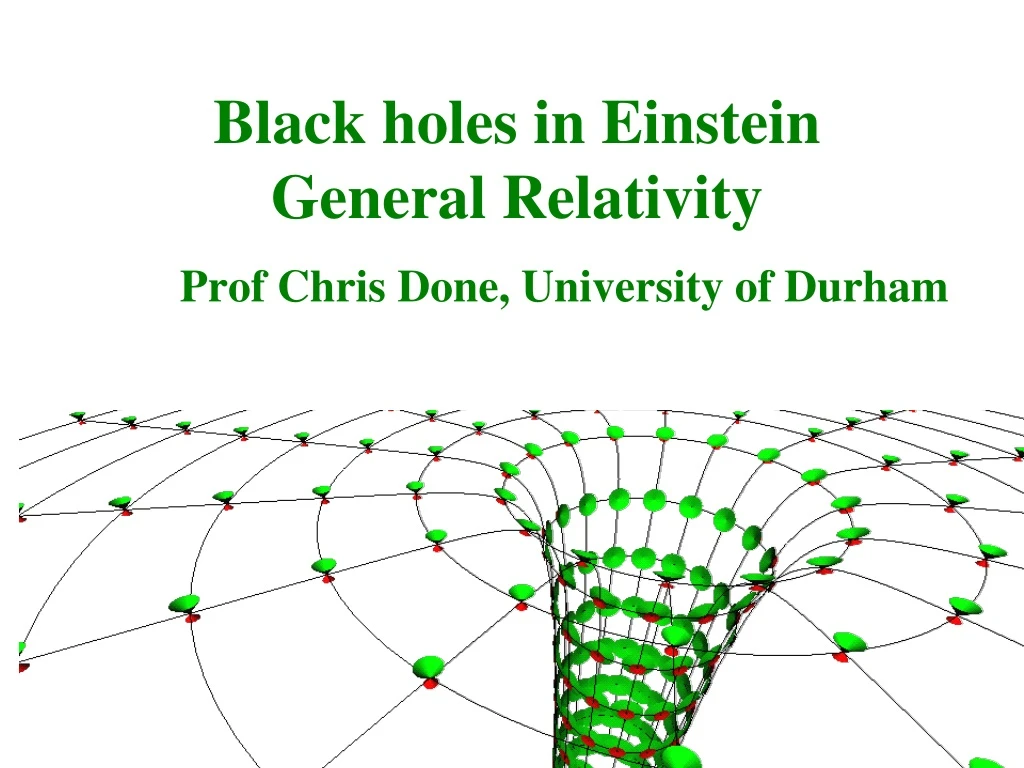
Black holes in Einstein General Relativity. Prof Chris Done, University of Durham. Lecture 1-2 recap:. Size in units of Rg = GM/c 2 = 1.5 10 5 M/M cm a=0, R H =2Rg, R isco =6Rg: a=0.998 R H ~ Rg , R isco =1.23Rg Gravity energy L ~ GM dM / dt = h( a ) dM / dt c 2

E N D
Black holes in EinsteinGeneral Relativity Prof Chris Done, University of Durham
Lecture 1-2 recap: Size in units of Rg= GM/c2 = 1.5 105M/M cm a=0, RH=2Rg, Risco=6Rg: a=0.998 RH~Rg, Risco=1.23Rg Gravity energy L ~ GM dM/dt = h(a)dM/dt c2 2Rin EddingtonLedd=4cpGM/sT=1.3 1038 M/M ergs/s
Variability of disc:long timescale • L/LEddAT4maxConstant size scale – last stable orbit!! • TAIL!! What is this??
Spectral states • Disc dominated - look like a disc but small tail to high energies • Very high/intermediate states at least know something about a disc • Low/hard state look really different, not at all like a disc! very high disk dominated high/soft Gierlinski & Done 2003
Variability of disc: short timescale • Timescale to change mass accretion rate through disc • tvisc= a-1 (H/R)-2torb =5 a-1 (H/R)-2 (r/6) -3/2ms • ~ 500s at last stable orbit for 10M • No rapid variability of disc 0.5 1.0 2.0
Low/hard state variability • Low/Hard state variability down to few 10s of ms • tvisc= a-1 (H/R)-2tdyn = 5 a-1 (H/R)-2 (r/6) -3/2ms • IF viscous timescale then H/R~1 0.5 1.0 2.0
Accretion flows without discs • Low L/Ledd: another stable solution of accretion flow • Hot, optically thin, geometrically thick inner flow replacing the inner disc (Shapiro et al. 1976; Narayan & Yi 1995- ADAF) • No disc so seed photons for compton from thermal electrons spiraling round B field (cyclo-sync) Log nfv(n) Log n
Radiation processes to get high energy radiation ACCRETION FLOW Thermal Comptonisation (BHB+AGN) Cyclo-synchrotron from thermal electrons JETS!! Synchrotron from Nonthermal electrons Comptonisation from Non-thermal electrons
Compton scattering theory eout ein • Collision – redistribute energy • If photon energy bigger than electron then it loses energy – downscattering • If photon has less energy than electron then it gains energy – upscattering qie qoe g qio
Compton scattering theory eout ein • Easiest to talk about if scale energies to mc2 so electron energy gmc2 just denoted g while photon energy becomes e=hn/mc2=E/511 for E (keV) qie qoe g qio eout = ein(1 - bcos qei) 1- bcos qeo+ (ein/g) (1- cosqio)
How much energy ? • Compton scattering seed photons from accretion disk. Photon energy boosted by factor De/e ~ 4Q+16Q2if thermal in each scattering.
Process cross-section s. Sweep out volume s R Number of particles in that volume is n s R = t How many scatterings? s cm2
How much scattering ? • Determined by optical depth, t=snR • Scattering probability exp(-t) • Optically thin t << 1 prob ~ t average number ~ t • Optically thick t>>1 prob~1 • average number ~ t2 R
How much total energy exchange? • Total fractional energy gain = frac.gain in 1 scatt x no.scatt • y = (4Q+16Q2) (t+t2 ) ~ 4Qt2 for Q<1 t>1 • y>1 flat spectrum • y<1 steep spectrum R
Optically thin thermal compton • power law by multiple scattering of thermal electrons • Compton scattering conserves photon number • Number of photons dN/dEdE = E dN/dEdLog E = f (e) dlogE • For t<1 scatter t photons each time to energy eout=(1+4Q+16Q2)ein Log fn Log N(g) Log g Log n
Optically thin thermal compton • For t<1 scatter t photons each time to energy eout=(1+4Q+16Q2)ein Log fn Log N(g) Log g Log n
Optically thin thermal compton • For t<1 scatter t photons each time to energy eout=(1+4Q+16Q2)ein Log fn Log N(g) Log g Log n
Optically thin thermal compton • For t<1 scatter t photons each time to energy eout=(1+4Q+16Q2)ein • Makes power law F(E) = A E-aas same fractional energy gain and same fraction of photons scattered Log fn Log N(g) Log g Log n
Question • Find the spectral index from F(E) = A E-a • Hint: first scattering is at E1, F1, second peaks at E1 (1+4Q+16Q2) and F1 t Log fn Log N(g) Log g Log n
Answer • F1= A E1-a • F2 = A E2-a but F2=F1 t and E2=E1 (1+4Q+16Q2) so F1 t= A E1-a (1+4Q+16Q2) -a divide and get a=-log t/log (1+4Q+16Q2) Log fn Log N(g) Log g Log n
Practice!! Mystery object • Estimate alpha, Q and t Log EF(E) 1 10 100 Log E (keV)
Spectra • Plot nf(n) as this peaks at energy where power output of source peaks. • N(E)=AE -G • F(E)=EN(E)= AE-G+1=AE-a a=G-1 LogEf(E)E) hard spectrum Most power at high E a<1 G<2 Log E dL= F(E) dE = EF(E) dE/E = EF(E) dlog E dN= N(E) dE = EN(E)dE/E = F(E) dlogE
Spectra • Plot nf(n) as this peaks at energy where power output of source peaks. • N(E)=AE -G • F(E)=EN(E)= AE-G+1=AE-a a=G-1 Log Ef(E) Soft spectrum Most power at low E a>1 G>2 Log E dL= F(E) dE = EF(E) dE/E = EF(E) dlog E
Optically thin thermal compton • Spectral index the same for different Q, t Log fn Log N(g) Log g Log n
Optically thin thermal compton • Spectral index the same for different Q, t • But spectrum goes bumpy for high Q Log fn Log N(g) Log g Log n
Spectral transitions in BHB Comptonised spectrum Tail is NONTHERMAL comptonisation !! Gierlinski et al 1999
And B fields • Generally there will be some B field • the thermal electrons can spiral around the B field lines - cyclotron radiation Q <<1 • cyclo-synchrotron if Q close to 1 or above • vB= eB/(2πmec) = 2.6x10⁶ B Hz Chiang & Done 2009
And B fields • Steep spectrum with exponential cutoffν~ νBθ2 • So much lower than electron temperature itself! Log vfn Log n Chiang & Done 2009
And B fields • But strongly self absorbed – electrons in the vicinity of a B field will absorb radiation • These can be the seed photons for comptonisation Log vfn Log n Chiang & Done 2009
And B fields • Black hole binary – optical and x-rays join up, so probably cyclo-synchrotron in the optical as the seed photons for thermal comptonisation Chiang et al 2010 Log vfn
Accretion flows without discs • Low L/Ledd: another stable solution of accretion flow • Hot, optically thin, geometrically thick inner flow replacing the inner disc (Shapiro et al. 1976; Narayan & Yi 1995- ADAF) Log nfv(n) Log n
Accretion flows without discs • Large scale height flow = large scale height B field close to horizon – jet !! • NOT the G=15 jets seen in blazars – these have G~1.5! Log nfv(n) Log n
Accretion flows – Jet Low/hard High/soft Very high Corbel et al 2012
Spectral transitions in BHB Disk dominated Comptonised spectrum Gierlinski et al 1999
Accretion flows – Jet Chaty et al 2003
AGN/QSO Zoo!!! Radio loud • Enormous, powerful, relativistic jets on Mpc scales • FRI (fuzzy) - BL lacs FRII (hot spots) – FSRQ • Urry & Padovani 1992; 1995
FRI is top of ADAF branch (low/hard state BHB) but G=15! L/LEdd BHB Ghisellini et al 2010
Optically thin nonthermal compton • power law by single scattering of nonthermal electrons N (g) g-p • index a = (p-1)/2 (p >2 so a > 0.5 – monoenergetic injection) • Starts a factor t down from seed photons, extends to gmax2ein ein eout~g2ein f(e) e-a e-(p-1)/2 g Log fn Log N(g) N (g) g-p Log g gmax gmax2ein ein Log n
Nonthermal synchrotron • power law by single scattering of nonthermal electrons N (g) g-p • index a = (p-1)/2 (p >2 so a > 0.5 – monoenergetic injection) • Starts a factor t down from seed photons, extends to gmax2ein ein eout~g2ein f(e) e-a e-(p-1)/2 g Log fn Log N(g) N (g) g-p Log g gmax gmax2ein ein Log n
Synchrotron self compton • Put in vfv • Expect index a = (p-1)/2~0.6 for p=2.2 from shocks Log vfn gmax gmax2ein ein Log n
Synchrotron self compton • Klein nisinacutoff – can’t have more energy than electron had to start with g2 hn < g mc2 so ge< 1 where e=hn/mc2 • Synchrotron self absorption Log vfn gmax gmax2ein ein Log n
Synchrotron self compton • Klein nisinacutoff – can’t have more energy than electron had to start with g2 hn < g mc2 so ge< 1 where e=hn/mc2 • Synchrotron self absorption Log vfn gmax gmax2ein ein Log n
Synchrotron self compton • Doppler boosting due to bulk motion G (don’t confuse with lorentz factor of electrons g) – d = 1/[G(1-bcosq)] • Eobs=Eintd • Fobs=Fintd3+a Log vfn gmax gmax2ein ein Log n
Synchrotron self compton • What we see in BL Lacs (Tavecchio et al 2010) Log vfn
BL Lacs as SSC • need G ~ 10-20, q<5o, gmax~105double power law electron distribution • Can’t make FSRQ Ghisellini et al 2010
Broad line region • AGN: complex environment • Scatters disc radiation
FSRQ –disc and BLR • Disc is behind jet so strongly deboosted • BLR may be much more isotropic so these external seed photons can be more important self produced synchrotron Ghisellini et al 2009
FSRQ –disc and BLR • Disc is behing jet so strongly deboosted • BLR may be much more isotropic so these external seed photons can be more important self produced synchrotron Log vfn gmax gmax2ein ein Log n Ghisellini et al 2009
FSRQ –disc and BLR • need G ~ 10-20, q<5o, gmax~105 double power law electron distribution similar to BL Lacs Log vfn gmax gmax2ein ein Log n Ghisellini et al 2009