Download
1 / 45
450 likes | 526 Vues
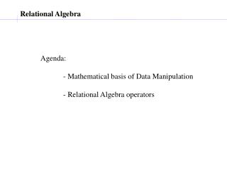
Relational Algebra. Procedural language Six basic operators select: project: union: set difference: – Cartesian product: x rename: closure. Select Operation. Notation: p ( r ) p : selection predicate Defined as: p ( r ) = { t | t r and p(t) }

E N D
Relational Algebra • Procedural language • Six basic operators • select: • project: • union: • set difference: – • Cartesian product: x • rename: • closure
Select Operation • Notation: p(r) • p : selection predicate • Defined as:p(r) = {t | t rand p(t)} p: a formula in propositional calculusconsisting of termsconnected by : , , Each term is one of: <attribute> op <attribute> or <constant> Op : =, , >, . <. • Example of selection:city=“mashad”(S)
A B C D 1 5 12 23 7 7 3 10 Relation r A B C D • A=B ^ D > 5(r) 1 23 7 10
Project Operation • Notation: where A1, A2 are attribute names and r is a relation name. • Duplicate rows removed from result, since relations are sets
A B C 10 20 30 40 1 1 1 2 • Relation r: A C A C 1 1 1 2 1 1 2 = A,C (r)
Union Operation • Notation: r s • Defined as: r s = {t | t r or t s} • For r s to be valid. 1. r,s must have the same arity (same number of attributes) 2. The attribute domains must be compatible
A B A B • Relations r, s: 1 2 1 r s 2 3 A B 1 2 1 3 r s:
Set Difference Operation • Notation r – s • Defined as: r – s = {t | t rand t s} • compatible relations: • r and s must have the samearity • attribute domains of r and s must be compatible
A B A B • Relations r, s: 1 2 1 2 3 s r A B 1 1 r – s:
Cartesian-Product Operation • Notation r x s • Defined as: r x s = {t q | t r and q s} • Assume that attributes of r(R) and s(S) are disjoint. • If attributes of r(R) and s(S) are not disjoint, then renaming must be used.
Relations r, s: C D E A B 10 10 20 10 a a b b 1 2 s r A B C D E 1 1 1 1 2 2 2 2 10 10 20 10 10 10 20 10 a a b b a a b b r xs:
Rename Operation • Allows us to name, and therefore to refer to, the results of relational-algebra expressions. • Allows us to refer to a relation by more than one name.
Additional Operations • do not add any power to the relational algebra, but that simplify common queries. • Set intersection • Natural join • Division • Assignment
Set-Intersection Operation • Notation: r s • Defined as: • rs = { t | trandts } • Assume: • r, s have the same arity • attributes of r and s are compatible
Relation r, s: A B A B 1 2 1 2 3 r s A B 2 r s
Natural-Join Operation Notation: r s R1 JOIN R2
r s B D E A B C D • Relations r, s: 1 3 1 2 3 a a a b b 1 2 4 1 2 a a b a b r s A B C D E 1 1 1 1 2 a a a a b
Division Operation r s • Notation: • Suited to queries that include the phrase “for all” . R = (A1, …, Am , B1, …, Bn) S = (B1, …, Bn) R S = (A1, …, Am) r s = { t | t R-S (r) u s (tu r ) }
Relations r, s: A B 1 2 3 1 1 1 3 4 6 1 2 B A 1 2 s r s: r
Relations r, s: A B C D E a a a a a a a a a a b a b a b b 1 1 1 1 3 1 1 1 A B C D E a a a b 1 1 s r s: r
Assignment Operation • provides a convenient way to express complex queries. • Write query as a sequential program consisting of a series of assignments • to a temporary relation variable. • Example: temp1 R-S (r )temp2 R-S ((temp1 x s ) – R-S,S (r ))result = temp1 – temp2
Extended Relational-Algebra-Operations • Extend and Summarize • Outer Join
Banking Example branch (branch_name, branch_city, assets) customer (customer_name,customer_street,custom_city) account (account_number, branch_name, balance) loan (loan_number, branch_name, amount) Depositor (customer_name,account_number) borrower (customer_name, loan_number)
Aggregate Functions and Operations • Aggregation function takes a collection of values and returns a single value as a result. avg: average valuemin: minimum valuemax: maximum valuesum: sum of valuescount: number of values
Aggregate operation in relational algebra E is any relational-algebra expression • G1, G2 …, Gn is a list of attributes on which to group (can be empty) • Each Fiis an aggregate function • Each Aiis an attribute name
Example: 1) Relation r: A B C 7 7 3 10 sum(c ) gsum(c) (r) 27
branch_name account_number balance 2) Relation account grouped by branch-name: Perryridge Perryridge Brighton Brighton Redwood A-102 A-201 A-217 A-215 A-222 400 900 750 750 700 branch_nameg sum(balance) (account) branch_name sum(balance) Perryridge Brighton Redwood 1300 1500 700
Result of aggregation does not have a name • Can use rename operation to give it a name • we permit renaming as part of aggregate operation branch_nameg sum(balance) assum_balance(account)
Extend • EXTEND term ADD scalar-expression AS attribute • (EXTEND PADD(WEIGHT*454) ASGMWT) WHERE GMWT>1000
Summarize • SUMMARIZE term BY (attribute-commalist)ADDaggregate-expressionAS attribute • SUMMARIZE (P JOIN SP) BY (CITY) ADD COUNT AS NSP • SUMMARIZE SP BY (P#) ADD SUM(QTY) AS TOTQTY,AVG(QTY) AS AVGQTY
Outer Join • An extension of the join operation that avoids loss of information. • Computes the join and then adds tuples from one relation that does not match tuples in the other relation to the result of the join. • Uses null values(unknown or does not exist )
branch_name loan_number amount Downtown Redwood Perryridge L-170 L-230 L-260 3000 4000 1700 customer_name loan_number Jones Smith Hayes L-170 L-230 L-155 Example • Relation loan Relation borrower
loan_number branch_name amount customer_name L-170 L-230 Downtown Redwood 3000 4000 Jones Smith Left Outer Join loan Borrower loan_number branch_name amount customer_name L-170 L-230 L-260 Downtown Redwood Perryridge 3000 4000 1700 Jones Smith null Example Inner Joinloan Borrower
Right Outer Join loan borrower loan_number branch_name amount customer_name L-170 L-230 L-155 Downtown Redwood null 3000 4000 null Jones Smith Hayes Full Outer Join loan borrower loan_number branch_name amount customer_name L-170 L-230 L-260 L-155 Downtown Redwood Perryridge null 3000 4000 1700 null Jones Smith null Hayes Example
Null Values • null signifies an unknown value or that a value does not exist. • The result of any arithmetic expression involving null is null. • Aggregate functions simply ignore null values • Comparisons with null values return the special truth value: unknown
Modification of the Database • operations: • Deletion • Insertion • Updating • All these operations are expressed using the assignment operator.
Deletion r r – E where r is a relation and E is a relational algebra expression. SP:=SP MINUS {{<s#:’s1’>,<p#:’p3’>,<qty:200>}}
Insertion r r E where r is a relation and E is a relational algebra expression. SP:=SP UNION {{<s#:’s4’>,<p#:’p2’>,<qty:150>}}
Updating UPDATE target assignment–commalist Attribute:=scalar-expression UPDATEpwhere color=‘red’ city:=‘mashad’
مقايسه هاي رابطه اي • expression Θ expression • Where Θ : <> = ≥ > ≤ < S[city] = P[city] S[s#] > SP[s#]
حساب رابطهاي حساب رابطهاي، با جبر رابطهاي منطقا معادل است، يعني براي هر عبارت جبر رابطهاي، يك عبارت معادل در حساب رابطهاي وجود دارد و برعكس. تفاوت آنها اين است كه جبر رابطهاي، دستوري است، اما حساب رابطهاي توصيفي است.
حساب تاپلي: در اين حساب مفهوم مهمي به نام متغير تاپلي وجود دارد كه تنها مقادير مجازش، تاپلهاي رابطه هستند. • حساب ميداني: در اين حساب، متغير ميداني وجود دارد كه از يك ميدان مقدار ميگيرد. در اين حساب يك شرط اضافي به نام شرط عضويت وجود دارد.
سور (Quantifier) 1-سور وجودي: به صورت نوشته ميشود، به اين معنا كه حداقل يك مقدار براي متغير T وجود دارد به نحوي كه f به ”درست“ ارزيابي شود. 2- سور همگاني: به صورت نوشته ميشود. يعني به ازای تمام مقادير متغير T، f به ”درست“ ارزيابي ميشود.
شكل كلي يك عبارت حساب رابطه اي تاپلي ( target-item (s) ) [ WHERE f]