Download
1 / 35
350 likes | 443 Vues
Mesoscale Cloud Climatologies. Ken Gould National Weather Service Tallahassee, FL Presented SatMet 00-1 Wednesday, 5 April 2000. Outline. Introduction Types of mesoscale cloud climatologies Channels used Stratification and averaging interval Applications Data integration

E N D
Mesoscale Cloud Climatologies Ken Gould National Weather Service Tallahassee, FLPresented SatMet 00-1Wednesday, 5 April 2000
Outline • Introduction • Types of mesoscale cloud climatologies • Channels used • Stratification and averaging interval • Applications • Data integration • Climatology design • Lab on sea breeze climatology over the Florida Panhandle
Introduction • Cloud climatologies began in the late 1960’s with analog cloud mosaics • Digital data gained use in the late 1970’s through the 1980’s • However, storage requirements and lack of computing power limited the development of cloud climatologies to the major universities and research centers
Now, mesoscale cloud climatologies can easily and inexpensively be done locally • Advent of the GOES 8/9/10 series • Increased PC and Workstation storage and CPU speed • Facilitated transmission of digital satellite data over the internet. A Direct Readout Ground Station is no longer a requirement to receive near real time data.
Types of Mesoscale Cloud Climatologies (MCC’s) • General- year round digital averaging of images at the same time and time interval • If in an area of infrequent change (equatorial regions), may be a good starting point. Otherwise, not recommended. • Seasonal- digital averaging of images at the same time and time interval over a particular season • Highly recommended. Allows for sufficient change in synoptic patterns, while still not requiring an inordinate amount of time to build a significant data base.
Monthly- digital averaging of images at the same time and time interval over each month • Also highly recommended. Provides more detail than seasonal in areas of frequent change. • However, may take several years to establish a significant data base, especially if a large number of regimes is used. • Phenomenon driven- used specifically to observe recurring phenomena over one’s area. May also be monthly, seasonal, or have some overlap. • Probably the best approach to an MCC. Requires the most insight and pre-planning, but should give the best results. Some examples include: • Sea Breeze • Fog/ sea fog/ stratus • Orographic
Channels • Visible- 1.1 km or 4 km
Stratification and Averaging Interval • Depending on the type of climatology and intended application, you may choose to stratify the data into regimes based on an appropriate synoptic flow. • For most applications, a low level wind or low Mean Layer Vector Wind (MLVW) at some chosen time of day should be used. For example, we use the 12 UTC MLVW from 1000 ft to 700 mb for the Florida Panhandle sea breeze climatology. • Note: SFC winds should generally be avoided since they may contain mesoscale contamination.
Regime development - several approaches possible • 8 pt. Compass --> 8 regimes • Onshore/offshore/parallel to shore flow • Upslope/downslope/parallel to slope flow • Bin by repetitive synoptic patterns during a particular season • Incorporate flow strengths • Eliminate “disturbed” days • Remember: the more regimes you choose, the more detailed your climatology will be, but the longer it will take to build a significant data base • Averaging Interval • Dependent on application • With GOES 8/9/10, 15 minute intervals possible • Generally hourly to 3 hourly recommended
Synoptic Flow Regimes and # of Days from the Summers of 1995-1997
Applications • Learn more about the phenomenon being studied and its behavior in a particular area • Can be used to help solve a myriad of forecast problems
Shows preferred areas of convective development 21 UTC image from regime 1, light and variable to light SE flow
Shows effects of synoptic flow changes on these preferred areas 20 UTC image from regime 2 (light to moderate E to NE flow) on left, 20 UTC image from regime 5 (strong W to SW flow) on right
May show marked effects from small scale features such as bays, lakes, and rivers 18 UTC image from regime 8 (light to moderate N to NW flow)
Shows preferred areas of fog/ low cloud development • Gives us insight into the timing of cloud development • Cloud frequency and probability tables can also be generated (Hall, et al., 1998) • Can be used as a direct aid in many NWS forecast products • Aviation forecasts (tafs and twebs) • Zone forecasts • Marine forecasts • Nowcasts
Data Integration- creates powerful forecast tools • Integration of complementary mesoscale climatologies • Precipitation • Probability of Precipitation (POP) • Radar (Hourly Digital Precipitation (HDP) data) • Lightning • Thermodynamic • Use of mesoscale models • Idealized runs • Real time modeling
Precipitation and POP • Precipitation and POP for Tallahassee by regime for 1995-1997
POP isopleths for regime 1 using Co-op sites over the Florida Panhandle
Lightning • Lightning flash density at 20 UTC for Regime 1
Thermodynamic • Use 12 UTC soundings from TLH • Modify soundings to expected 18 UTC conditions using SHARP Workstation • Average levels every 50 mb for both modified and unmodified soundings for each regime • Analyze the mean soundings and convective parameters such as CAPE and PW
Mesoscale Models • Here at NWSO TAE, we use the non-hydrostatic version of the PSU/NCAR MM5 run on an HP-755 • Initialize with the eta/meso eta for course grid boundary conditions • Run operationally twice a day at 15 km horizontal resolution • Output from operational runs can be viewed on the web at: http://www.nws.fsu.edu/tlh/mm5 • Idealized runs • Run nested at 15/5 km horizontal resolution • Initialized with low level flows from climatology • Initialized with 12 UTC unmodified soundings from climatology
Climatology Design • Choose type or types • Choose channels and products • Choose synoptic flow stratification • Integrate complementary climatologies and mesoscale modeling • Test in forecast situations
Suggested Reading • Klitch, M.A., J.F. Weaver, F.P. Kelly, and T.H. Vonder Haar, 1985: Convective cloud climatologies constructed from satellite imagery. Mon. Wea. Rev.,113, 326-337. • Gibson, H.M., and T.H. Vonder Haar, 1990: Cloud and convection frequency over the southeast United States as related to small scale geographic features. Mon. Wea. Rev., 118, 2215-2227. • Hall, T.J., D.L. Reinke, and T.H. Vonder Haar, 1998: Forecasting applications of high resolution satellite cloud composite climatologies. Wea. and For., 13, 16-23. • Gould, K.J., and H.E. Fuelberg, 1996: The use of GOES-8 imagery and RAMSDIS to develop a sea breeze climatology over the Florida Panhandle. Preprints, 8th Conf. On Satellite Meteorology and Oceanography, 100-104.
Questions • 1. Weighing all of the advantages and disadvantages, which type of mesoscale cloud climatology is probably the best? • a. General • b. Seasonal • c. Monthly • d. Seasonal Phenomenon Driven • e. Monthly Phenomenon Driven
2. Name three examples of a phenomenon driven MCC • 3. If performing a phenomenon driven MCC for wild fires/prescribed burns, what two GOES 8/10 channels would be best to use? • a. Water vapor/ 3.9 micron IR • b. 10.7 micron IR/ visible • c. Fog product/ 10.7 micron IR • d. 3.9 micron IR/ visible • e. Visible/ water vapor
4. In developing a stratification scheme based on the low level synoptic flow, why should the surface wind generally be avoided? • 5. How would an MCC be used as an aid in the following NWS forecast products: • a. Aviation forecasts? • b. Zone forecasts? • c. Marine forecasts?
6. Name three complementary mesoscale climatologies one might use in conjunction with an MCC. • 7. How could precipitation climatologies be used when composing a zone forecast? • 8. Besides a sea breeze climatology, what other phenomenon driven MCC might be served well by a thermodynamic climatology?
Answers • 1. d. A monthly phenomenon driven MCC would also be good, but it would take much longer to build a significant data base. • 2. Sea breeze, fog/sea fog/stratus, orographic, fire • 3. d. • 4. The surface wind should generally be avoided since it may contain mesoscale contamination. For example, in determining the synoptic flow for a sea breeze climatology, the surface wind may contain a component of the land or sea breeze which is non-representative of the synoptic flow. • 5. a. An MCC will give an excellent first guess of the timing and preferred locations of the development and dissipation of clouds and fog. • b. As in a., in addition to, likely areas of precipitation and convective development. This may help determine zone grouping. • c. Similar to a., with emphasis on sea fog and stratus.
Answers (cont.) • 6. Precipitation, POP, Radar (HDP), Lightning, Thermodynamic. • 7. Precipitation climatologies could be used as an excellent first guess for grouping zones by probability of precipitation (POP), in addition to a rough first guess of QPF. Also, the HDP data can be used as a verification tool for both zone and QPF forecasts. • 8. A fog/sea fog/stratus MCC should be well served by a thermodynamic climatology. The mean sounding structure should be a good indicator of days with or without fog/sea fog/stratus. In fact, with a well stratified thermodynamic climatology, one might even be able to delineate fog/sea fog vs. stratus. (one of the more challenging forecast problems)