Download

1 / 62
620 likes | 810 Vues
Lecture 8: Stereo. X. z. x. x’. f. f. Baseline B. C. C’. Depth from Stereo. X. Goal: recover depth by finding image coordinate x’ that corresponds to x. x. x'. X. z. x. x’. f. f. Baseline B. C. C’. Depth from Stereo. X.

E N D
X z x x’ f f BaselineB C C’ Depth from Stereo X • Goal: recover depth by finding image coordinate x’ that corresponds to x x x'
X z x x’ f f BaselineB C C’ Depth from Stereo X • Goal: recover depth by finding image coordinate x’ that corresponds to x • Problems • Calibration: How do we recover the relation of the cameras (if not already known)? • Correspondence: How do we search for the matching point x’? x x'
Correspondence Problem • We have two images taken from cameras at different positions • How do we match a point in the first image to a point in the second? What constraints do we have?
A pre-sequitor • Fun with vectors. Let a and b be two vectors. • What is a (dot) b? • What is a (cross) b? Quiz: • What is a (dot) a? • (what is the data type?) • What is a (cross) a?
Recap, Camera Calibration. • Projection from the world to the image: Calibration Rotation Translation Homogeneous equal, “equal up to a scale factor” Computer Vision, Robert Pless
Idea of today… • Today we are going to characterize the geometry of how two cameras look at a scene… but perhaps a more complicated. • And by scene, we mean, at first, just one point. Computer Vision, Robert Pless
Epipolar Constraint There are 3 degrees of freedom in the position of a point in space; there are four DOF for image points in two planes… Where does that fourth DOF go? Computer Vision, Robert Pless
Epipolar Lines Potential 3d points Red point - fixed => Blue point lies on a line Each point in one image corresponds to a line of possibilities in the other. “Epipolar Line” Computer Vision, Robert Pless
Epipolar Geometry => Red point lies on a line baseline Blue point - fixed An epipole is the image point of the other camera’s center. All epipolar lines meet at the epipoles. Epipoles lie on the cameras’ baseline. Computer Vision, Robert Pless Is there other structure available among epipolar lines?
Another look (with math). • We have two images, with a point in one and the epi-polar line in the other. Lets take away the image plane, and just leave the image centers. Computer Vision, Robert Pless
Another look (with math). Computer Vision, Robert Pless
Another look (with math). a translation vector defining where one camera is relative to the other. Computer Vision, Robert Pless
Another look (with math). a translation vector defining where one camera is relative to the other. Computer Vision, Robert Pless
Another look (with math). A point on one image lies on ray in space with direction Computer Vision, Robert Pless
Another look (with math). • Which rays from, the second camera center might intersect ray p? Computer Vision, Robert Pless
Another look (with math). • Those rays lie in the plane defined by the ray in space and the second camera center. Computer Vision, Robert Pless
Another look (with math). - • normal of the plane is perpendicular to both p and t. • Math fact: a x b is a vector perpendicular to a and b. Computer Vision, Robert Pless
Another look (with math). • All lines in the plane are perpendicular to the normal to normal to the plane. • Math fact. aTb = 0 if a is perpendicular to b Computer Vision, Robert Pless
Putting it all together. Fact: • Cameras separated by translation t • Ray from one camera center in direction p • Ray from second camera center q Computer Vision, Robert Pless
Lets put the images back in. y x P is relative to some coordinate system. Computer Vision, Robert Pless
x y x y • q is relative to some coordinate system, but that camera may have rotated. • So the q in the first coordinate system is some rotation times the q measured in the second coordinate system Computer Vision, Robert Pless
x y x y • All three vectors in the same plane: Computer Vision, Robert Pless
Put images even more back in. (x,y) • K maps normalized coordinates onto pixel coordinates. Given pixel coordinates (x,y), K-1 remaps those to a direction from the camera center. Computer Vision, Robert Pless
Normalized camera system, epipolar equation. “Uncalibrated” Case, epipolar equation: F is the “fundamental matrix”. Computer Vision, Robert Pless
Using the equation… • Click on “the same world point” in the left and right image, to get a set of point correspondences: (x,y) that correspond to (x’,y’). • Need at least 8 points (each point gives one constraint, F is 3x3, but scale invariant, so there are 8 degrees of freedom in F). Computer Vision, Robert Pless
So what… how to use F Potential 3d points Red point - fixed => Blue point lies on a line Given a point (x,y) on the left image, F defines the “Epipolar Line” and tells where the corresponding points must lie. How is that line defined? Only easy in homogenous coordinates! Computer Vision, Robert Pless
Examples Computer Vision, Robert Pless http://www-sop.inria.fr/robotvis/personnel/sbougnou/Meta3DViewer/EpipolarGeo.html
Examples Computer Vision, Robert Pless
Examples Computer Vision, Robert Pless Geometrically, why do all epipolar lines intersect?
Estimating the Fundamental Matrix • 8-point algorithm • Least squares solution using SVD on equations from 8 pairs of correspondences • Enforce det(F)=0 constraint using SVD on F • Minimize reprojection error • Non-linear least squares
8-point algorithm • Solve a system of homogeneous linear equations • Write down the system of equations
8-point algorithm • Solve a system of homogeneous linear equations • Write down the system of equations • Solve f from Af=0 using SVD Matlab: [U, S, V] = svd(A); f = V(:, end); F = reshape(f, [3 3])’;
8-point algorithm • Solve a system of homogeneous linear equations • Write down the system of equations • Solve f from Af=0 using SVD • Resolve det(F) = 0 constraint by SVD Matlab: [U, S, V] = svd(A); f = V(:, end); F = reshape(f, [3 3])’; Matlab: [U, S, V] = svd(F); S(3,3) = 0; F = U*S*V’;
8-point algorithm • Solve a system of homogeneous linear equations • Write down the system of equations • Solve f from Af=0 using SVD • Resolve det(F) = 0 constraint by SVD Notes: • Use RANSAC to deal with outliers (sample 8 points) • Solve in normalized coordinates • mean=0 • RMS distance = (1,1,1) • This also help estimating the homography for stitching
Comparison of homography estimation and the 8-point algorithm Assume we have matched points x x’ with outliers Homography (No Translation) Fundamental Matrix (Translation)
Comparison of homography estimation and the 8-point algorithm Assume we have matched points x x’ with outliers Homography (No Translation) Fundamental Matrix (Translation) • Correspondence Relation • RANSAC with 4 points
Comparison of homography estimation and the 8-point algorithm Assume we have matched points x x’ with outliers Homography (No Translation) Fundamental Matrix (Translation) Correspondence Relation RANSAC with 8 points Enforce by SVD • Correspondence Relation • RANSAC with 4 points
So • Given 2 images. Can find the relative translation and rotations of the cameras. How do we find depth?
Simplest Case: Parallel images • Image planes of cameras are parallel to each other and to the baseline • Camera centers are at same height • Focal lengths are the same • Then, epipolar lines fall along the horizontal scan lines of the images
Depth from disparity X z x x’ f f BaselineB O O’ Disparity is inversely proportional to depth.
Stereo image rectification • Reproject image planes onto a common plane parallel to the line between camera centers • Pixel motion is horizontal after this transformation • Two homographies (3x3 transform), one for each input image reprojection • C. Loop and Z. Zhang. Computing Rectifying Homographies for Stereo Vision. IEEE Conf. Computer Vision and Pattern Recognition, 1999.
Basic stereo matching algorithm • If necessary, rectify the two stereo images to transform epipolar lines into scanlines • For each pixel x in the first image • Find corresponding epipolarscanline in the right image • Examine all pixels on the scanline and pick the best match x’ • Compute disparity x-x’ and set depth(x) = fB/(x-x’)
Correspondence search Left Right • Slide a window along the right scanline and compare contents of that window with the reference window in the left image • Matching cost: SSD or normalized correlation scanline Matching cost disparity
Correspondence search Left Right scanline SSD
Correspondence search Left Right scanline Norm. corr
Effect of window size W = 3 W = 20 • Smaller window + More detail • More noise • Larger window + Smoother disparity maps • Less detail