Download
1 / 15
150 likes | 225 Vues
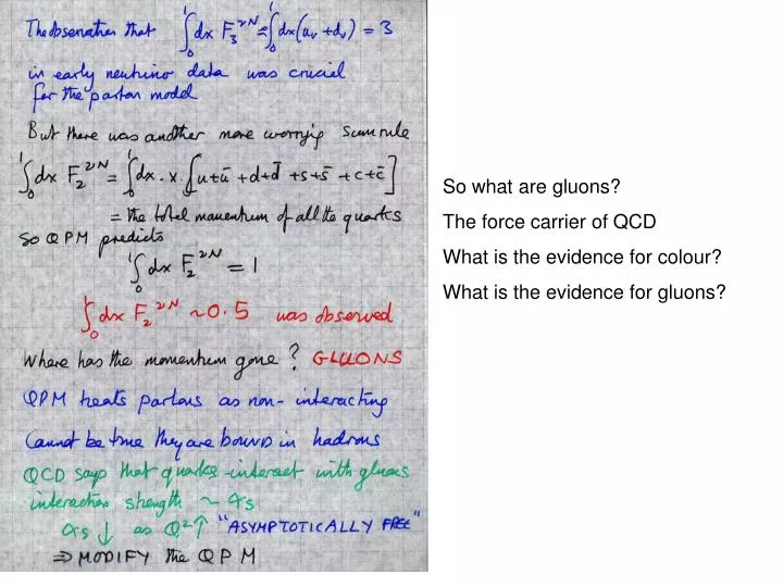
So what are gluons? The force carrier of QCD What is the evidence for colour? What is the evidence for gluons?. ATLAS 2010 A M Cooper-Sarkar Jan 2011. Gemma (Trigger representative for ATLAS Higgs group Sinead (VBF convenor for LHC cross-section working group)

E N D
So what are gluons? The force carrier of QCD What is the evidence for colour? What is the evidence for gluons?
ATLAS 2010A M Cooper-SarkarJan 2011 Gemma (Trigger representative for ATLAS Higgs group Sinead (VBF convenor for LHC cross-section working group) Elias (Editor of ATLAS Z →ττ documentation
QED (electrons and photons) QCD (quarks and gluons) And here are some pictures of quarks, gluons, electrons and photons from LEP @ CERN 1989-2000 e+ e- annihilation. Illustrating that partons behave similarly to the point-like electron and photon q e+ e- q e+ q γ e- q You don’t see the quark or gluon emerge instead you see a jet: a “blast” of particles, all going in roughly the same direction.
QCD is a locally gauge invariant field theory like QED For QED this means Where q is the charge and θ is a space-time dependent phase. The QED Lagrangian is with and The interaction between the fermions and the field is in the covaraint derviative For QCD Where g is the strong charge and t.θ is the product of the colour group generators with a vector of space-time phase functions in colour space. The group generators t satisfy Where fabc are SU(3) structure constants. f123=1, f147=f246=f257=f345=1/2,f156=f367=1/2,f458=f678=√3/2 The Gell-Mann λ matrices are given by The quark part of theQCD Lagrangian is With where taij are hermitian matrices = λaij /2. U(1) This describes the qqg interaction Where quarks now have colour indices i=1,2,3 (R,G,B) as well as flavour indices f. The gluon fields A have a=1-8 flavour indices...... SU(3)
The colour exchange in q q g diagram can be thought of like this SO the gluon has colour red- antigreen: r-gbar Obviously r-bbar, g-rbar, g-bbar, b-gbar, b-rbar are also possible and the combinations (r-rbar - g-gbar)/√2, (r-rbar + g-gbar – 2b-bar)/√6 and (r-rbar + b-bar + g-gbar)/√3 In the mathematics of SU(3) this is 3 * 3 = 8 + 1 And the last combination is the singlet– which is not coloured at all, hence eight coloured gluons (Think of SU(2) 2*2=3+1 -triplets and singlets- in atomic physics if this puzzles you) The second part of the QCD Lagrangian is purely gluonic Where The difference from QED is the A A term which is what makes gluons interact with gluons (NON-Abelian) with both a g-g-g vertex and a g-g-g-g vertex The colour flow is more complex for these vertices ~ twice as strong as for q-q-g This extra term is also what makes QCD gauge invariant under local SU(3) transformation
Perturbative QCD involves an order by order expansion in a small coupling αS = g2 /4π << 1 and calculations are made using Feynman diagrams. The rules for the vertices have already been shown. The main complication in comparison to QED is the need for colour factors. After squaring an amplitude and summing over colours of incoming and outgoing particles the colour factors often appear in one or other of the following combinations: Where the final diagram gives the Fierz indentity- a mathematical formulation of the colour flow. See page 38/39 Devenish and Cooper-Sarkar for a simple colour factor calculation
To go to QCD e4 must be replaced And the colour factor from the loop insertion CF=4/3 Consider QED Compton scattering with one virtual photon And using the Golden rule to got to the cross-section via the phase space factors The QCD analogue is QCDC and the kinematic invariants are A further important process is Boson-Gluon Fusion BGF The amplitudes for the two QED diagrams are Adding squaring and taking care of spins which, similarly, has the cross-section Devenish and Cooper-Sarkar p40-43
Contributions to the perturbative expansion of scattering amplitudes beyond the leading order are often divergent, e.g for QED For many loops the effect of summing the ‘leading logs’ can be accounted for by redefining the coupling We must remove the dependence on Λ and α0 by defining the coupling at some scale μ2 and writing its value at all other scales Q2 in terms of this (‘renomalisation’ ) Thus for Q2>μ2 the coupling increases And indeed the 1/137 you are used to at low energies becomes 1/125 at the scale of MZ2 This can be understood qualitatively in terms of charge screening What of QCD? The loops are divergent beacuse of unrestricted integration over momentum in these loops We have to renormalize the theory. This is done by making constants of the theory like the coupling α become dependent on the scale of the process. It is sucessful if this takes care of ALL the infinities to all orders. For one loop the fermion propagator becomes where Λ is a high momentum cut-off and α0 is the bare e.m. charge
What of QCD? There is another type of loop diagram. Both contributions diverge logarithmically but with opposite sign The QCD coupling is renormalised as Where at leading order. Note the quark loop gives 1/6π for each flavour of fermion (nf) – this is like the 1/3π of QED bar a convetional factor of 2. The new feacture is the 33/12π of the gluon loop which swaps the sign Gives us anti-screening Or ASMYPTOTIC FREEDOM The coupling decreases as the scale goes up At high energies we may make perturbative caluclations At low- energies we can’t and we have CONFINEMENT
Let us apply some of this to the parton model = and the γ*p cross-section is The convolution of a probability of finding a parton in the proton with a hard scattering cross-section. The γ*quark interaction cross-section is where so gives the QPM parton model result Now let’s add these diagrams The hard cross section here is just the QCDC diagrams so Where So if c=cosθ There are singularities at c=1, z=1. z=1 is an infra-red singluarity that is cancelled by other terms c=1 corresponds to the gluon being emitted collinearly. The residue at the pole is
Do the integration in terms of the gluon (or quark transverse momentum in the CMS Gives Where But the pt integral also needs a lower cut-off to regulate it so Essentially gluon radiation introduces non zero pt and integrating over it gives log terms. Define As the probability for a quark to split into a quark and a gluon then Where the log term is dominant. NOW add this term to the QPM result Redefine the parton density Where The next step is to ‘renormalise’ the parton density by choosing a factorisation scale at which to define the parton density Thus the bare parton density becomes a renormalised parton density which depends on the scale at which it is observed. The collinear singularity is absorbed into the parton density and if Q2=μ2 is the factorisation scale then
The renormalised parton density qi(x,μ2) cannot be calculated perturbatively (soft non perturbative physics has been absorbed into it) but we do know how it evolves with scale Except that we still have to add on the BGF processes And introducing an infra-red cut-off and a bare gluon density gives where Is the probaibility for a gluon to split into a q-qbar pair Regularising the cut-off in this extra contribution to F2 gives us an extra contribution to qi(x,μ2) such that its evolution with scale is given by where the extra term depends o a renormalised gluon denisty. The expression for F2 then remains as Writing the angular integral in terms of pt
Probable end lecture 2 So F2(x,Q2) = Σi ei2(xq(x,Q2) + xq(x,Q2)) in LO QCD And the theory predicts the rate at which the parton distributions (both quarks and gluons) evolve with Q2- (the energy scale of the probe) -BUT it does not predict their starting shape