Root finding Methods

1. Root finding Methods Solving Non-Linear Equations (Root Finding)

2. Root finding Methods • What are root finding methods? • Methods for determining a solution of an equation. • Essentially finding a root of a function, that is, a zero of the function.

3. Root finding Methods • Where are they used? • Some applications for root finding are: systems of equilibrium, elliptical orbits, the van der Waals equation, and natural frequencies of spring systems.

4. The problem of solving non-linear equations or sets of non-linear equations is a common problem in science, applied mathematics.

5. The problem of solving non-linear equations or sets of non-linear equations is a common problem in science, applied mathematics. • The goal is to solve f(x) = 0 , for the function f(x). • The values of x which make f(x) = 0 are the roots of the equation.

6. a,b are roots of the function f(x) f(a)=0 f(b)=0 f(x) x

7. More complicated problems are sets of non-linear equations. f(x, y, z) = 0 h(x, y, z) = 0 g(x, y, z) = 0

8. More complicated problems are sets of non-linear equations. f(x, y, z) = 0 h(x, y, z) = 0 g(x, y, z) = 0 • For N variables (x, y, z ,…), the equations are solvable if there are N linearly independent equations.

9. There are many methods for solving non-linear equations. The methods, which will be highlighted have the following properties: • the function f(x) is expected to be continuous. If not the method may fail. • the use of the algorithm requires that the solution be bounded. • once the solution is bounded, it is refined to specified tolerance.

10. Four such methods are: • Interval Halving (Bisection method) • Regula Falsi (False position) • Secant method • Fixed point iteration • Newton’s method

11. Bisection Method

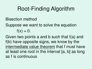
12. Bisection Method • It is the simplest root-finding algorithm. • requires previous knowledge of two initial guesses, a and b, so that f(a) and f(b) have opposite signs. initial pt ‘b’ a d c b root ‘d’ initial pt ‘a’

13. Bisection Method • Two estimates are chosen so that the solution is bracketed. ie f(a) and f(b) have opposite signs. • In the diagram this f(a) < 0 and f(b) > 0. • The root d lies between a and b! initial pt ‘b’ a d c b root ‘d’ initial pt ‘a’

14. Bisection Method • The root d must always be bracketed (be between a and b)! • Iterative method. initial pt ‘b’ a d c b root ‘d’ initial pt ‘a’

15. Bisection Method • The interval between a and b is halved by calculating the average of a and b. • The new point c = (a+b)/2. • This produces are two possible intervals: a < x < c and c < x < b. initial pt ‘b’ a d c b root ‘d’ initial pt ‘a’

16. Bisection Method • This produces are two possible intervals: a < x < c and c < x < b. • If f(c ) > 0, then x = d must be to the left of c :interval a < x < c. • If f(c ) < 0, then x = d must be to the right of c :interval c < x < b. initial pt ‘b’ a d c b root ‘d’ initial pt ‘a’

17. Bisection Method • If f(c ) > 0, let anew = a and bnew = c and repeat process. • If f(c ) < 0, let anew = c and bnew = b and repeat process. • This reassignment ensures the root is always bracketed!! initial pt ‘b’ a d c b root ‘d’ initial pt ‘a’

18. Bisection Method • This produces are two possible intervals: a < x < c and c < x < b. • If f(c ) > 0, then x = d must be to the left of c :interval a < x < c. • If f(c ) < 0, then x = d must be to the right of c :interval c < x < b. initial pt ‘b’ a d c b root ‘d’ initial pt ‘a’

19. Bisection Method ci = (ai + bi )/2 if f(ci) > 0; ai+1 = a and bi+1 = c if f(ci) < 0; ai+1 = c and bi+1 = b

20. Bisection Method • Bisection is an iterative process, where the initial interval is halved until the size of the interval decreases until it is below some predefined tolerance : |a-b|  or f(x) falls below a tolerance : |f(c ) – f(c-1)| .  

21. Bisection Method • Advantages • Is guaranteed to work if f(x) is continuous and the root is bracketed. • The number of iterations to get the root to specified tolerance is known in advance

22. Bisection Method • Disadvantages • Slow convergence. • Not applicable when here are multiple roots. Will only find one root at a time.

23. Linear Interpolation Methods

24. Linear Interpolation Methods • Most functions can be approximated by a straight line over a small interval. The two methods :- secant and false position are based on this.

25. Secant Method

26. Secant Method

27. Overview of Secant Method • Again to initial guesses are chosen. • However there is not requirement that the root is bracketed! • The method proceeds by drawing a line through the points to get a new point closer to the root. • This is repeated until the root is found.

28. Secant Method • First we find two points(x0,x1), which are hopefully near the root (we may use the bisection method). • A line is then drawn through the two points and we find where the line intercepts the x-axis, x2.

29. Secant Method • If f(x) were truly linear, the straight line would intercept the x-axis at the root. • However since it is not linear, the intercept is not at the root but it should be close to it.

30. Secant Method • From similar triangles we can write that,

31. Secant Method • From similar triangles we can write that, • Solving for x2 we get:

32. Secant Method • Iteratively this is written as:

33. Algorithm • Given two guesses x0, x1 near the root, • If then • Swap x0 and x1. • Repeat • Set • Set x0 = x1 • Set x1 = x2 • Until < tolerance value.

34. Because the new point should be closer the root after the 2nd iteration we usually choose the last two points. • After the first iteration there is only one new point. However x1 is chosen so that it is closer to root that x0. • This is not a “hard and fast rule”!

35. Discussion of Secant Method • The secant method has better convergence than the bisection method( see pg40 of Applied Numerical Analysis). • Because the root is not bracketed there are pathological cases where the algorithm diverges from the root. • May fail if the function is not continuous.

36. Pathological Case • See Fig 1.2 page 40

37. False Position

38. False Position

39. False Position • The method of false position is seen as an improvement on the secant method. • The method of false position avoids the problems of the secant method by ensuring that the root is bracketed between the two starting points and remains bracketing between successive pairs.

40. False Position • This technique is similar to the bisection method except that the next iterate is taken as the line of interception between the pair of x-values and the x-axis rather than at the midpoint.

41. False Position

42. Algorithm • Given two guesses x0, x1 that bracket the root, • Repeat • Set • If is of opposite sign to then • Set x1 = x2 • Else Set x0 = x1 • End If • Until < tolerance value.

43. Discussion of False Position Method • This method achieves better convergence but a more complicated algorithm. • May fail if the function is not continuous.

44. Newton’s Method

45. Newton’s Method • The bisection method is useful up to a point. • In order to get a good accuracy a large number of iterations must be carried out. • A second inadequacy occurs when there are multiple roots to be found.

46. Newton’s Method • The bisection method is useful up to a point. • In order to get a good accuracy a large number of iterations must be carried out. • A second inadequacy occurs when there are multiple roots to be found. • Newton’s method is a much better algorithm.

47. Newton’s Method • Newton’s method relies on calculus and uses linear approximation to the function by finding the tangent to the curve.

48. Newton’s Method • Algorithm requires an initial guess, x0, which is close to the root. • The point where the tangent line to the function (f (x)) meets the x-axis is the next approximation, x1. • This procedure is repeated until the value of ‘x’ is sufficiently close to zero.

49. Newton’s Method • The equation for Newton’s Method can be determined graphically!

50. Newton’s Method • The equation for Newton’s Method can be determined graphically! • From the diagram tan Ө = ƒ'(x0) = ƒ(x0)/(x0 – x1)