Download
1 / 79
790 likes | 990 Vues
Graphical Descriptive Techniques. 2.1 Introduction. Descriptive statistics involves the arrangement, summary, and presentation of data, to enable meaningful interpretation, and to support decision making. Descriptive statistics methods make use of graphical techniques

E N D
2.1 Introduction • Descriptive statistics involves the arrangement, summary, and presentation of data, to enable meaningful interpretation, and to support decision making. • Descriptive statistics methods make use of • graphical techniques • numerical descriptive measures. • The methods presented apply to both • the entire population • the population sample
2.2 Types of data and information • A variable - a characteristic of population or sample that is of interest for us. • Cereal choice • Capital expenditure • The waiting time for medical services • Data - the actual values of variables • Interval data are numerical observations • Nominal data are categorical observations • Ordinal data are ordered categorical observations
Types of data - examples Interval data Nominal Age - income 55 75000 42 68000 . . . . PersonMarital status 1 married 2 single 3 single . . . . Weight gain +10 +5 . . Computer Brand 1 IBM 2 Dell 3 IBM . . . .
Types of data - examples Interval data Nominal data With nominal data, all we can do is, calculate the proportion of data that falls into each category. Age - income 55 75000 42 68000 . . . . Weight gain +10 +5 . . IBM Dell Compaq Other Total 25 11 8 6 50 50% 22% 16% 12%
Types of data – analysis • Knowing the type of data is necessary to properly select the technique to be used when analyzing data. • Type of analysis allowed for each type of data • Interval data – arithmetic calculations • Nominal data – counting the number of observation in each category • Ordinal data - computations based on an ordering process
Cross-Sectional/Time-Series Data • Cross sectional data is collected at a certain point in time • Marketing survey (observe preferences by gender, age) • Test score in a statistics course • Starting salaries of an MBA program graduates • Time series data is collected over successive points in time • Weekly closing price of gold • Amount of crude oil imported monthly
2.3 Graphical Techniques for Interval Data • Example 2.1: Providing information concerning the monthly bills of new subscribers in the first month after signing on with a telephone company. • Collect data • Prepare a frequency distribution • Draw a histogram
Class width = [Range] / [# of classes] [119.63 - 0] / [8] = 14.95 15 Example 2.1: Providing information Collect data Prepare a frequency distribution How many classes to use? Number of observations Number of classes Less then 50 5-7 50 - 200 7-9 200 - 500 9-10 500 - 1,000 10-11 1,000 – 5,000 11-13 5,000- 50,000 13-17 More than 50,000 17-20 (There are 200 data points Smallest observation Largest observation Largest observation Largest observation Largest observation Smallest observation Smallest observation Smallest observation
Draw a Histogram Example 2.1: Providing information
Example 2.1: Providing information What information can we extract from this histogram Relatively, large number of large bills About half of all the bills are small A few bills are in the middle range 71+37=108 13+9+10=32 80 18+28+14=60 60 Frequency 40 20 0 15 45 75 30 60 90 105 120 Bills
Class frequency Total number of observations Class relative frequency = Relative frequency • It is often preferable to show the relative frequency (proportion) of observations falling into each class, rather than the frequency itself. • Relative frequencies should be used when • the population relative frequencies are studied • comparing two or more histograms • the number of observations of the samples studied are different
Class width • It is generally best to use equal class width, but sometimes unequal class width are called for. • Unequal class width is used when the frequency associated with some classes is too low. Then, • several classes are combined together to form a wider and “more populated” class. • It is possible to form an open ended class at the higher end or lower end of the histogram.
Shapes of histograms Symmetry • There are four typical shape characteristics
Shapes of histograms Skewness Negatively skewed Positively skewed
Modal classes A modal class is the one with the largest number of observations. A unimodal histogram The modal class
Modal classes A bimodal histogram A modal class A modal class
Bell shaped histograms • Many statistical techniques require that the population be bell shaped. • Drawing the histogram helps verify the shape of the population in question
Interpreting histograms • Example 2.2: Selecting an investment • An investor is considering investing in one out of two investments. • The returns on these investments were recorded. • From the two histograms, how can the investor interpret the • Expected returns • The spread of the return (the risk involved with each investment)
The center for A The center for B Example 2.2 - Histograms 18- 16- 14- 12- 10- 8- 6- 4- 2- 0- 18- 16- 14- 12- 10- 8- 6- 4- 2- 0- -15 0 15 30 45 60 75 -15 0 15 30 45 60 75 Return on investment A Return on investment B Interpretation:The center of the returns of Investment Ais slightly lower than that for Investment B
17 16 26 34 43 46 Example 2.2 - Histograms Sample size =50 Sample size =50 18- 16- 14- 12- 10- 8- 6- 4- 2- 0- 18- 16- 14- 12- 10- 8- 6- 4- 2- 0- -15 0 15 30 45 60 75 -15 0 15 30 45 60 75 Return on investment A Return on investment B Interpretation:The spread of returns for Investment Ais less than that for investment B
Example 2.2 - Histograms 18- 16- 14- 12- 10- 8- 6- 4- 2- 0- 18- 16- 14- 12- 10- 8- 6- 4- 2- 0- -15 0 15 30 45 60 75 -15 0 15 30 45 60 75 Return on investment A Return on investment B Interpretation:Both histograms are slightly positively skewed. There is a possibility of large returns.
Providing information • Example 2.2: Conclusion • It seems that investment A is better, because: • Its expected return is only slightly below that of investment B • The risk from investing in A is smaller. • The possibility of having a high rate of return exists for both investment.
Interpreting histograms • Example 2.3: Comparing students’ performance • Students’ performance in two statistics classes were compared. • The two classes differed in their teaching emphasis • Class A – mathematical analysis and development of theory. • Class B – applications and computer based analysis. • The final mark for each student in each course was recorded. • Draw histograms and interpret the results.
Interpreting histograms The mathematical emphasis creates two groups, and a larger spread.
2.5 Describing the Relationship Between Two Variables • We are interested in the relationship between two interval variables. • Example 2.7 • A real estate agent wants to study the relationship between house price and house size • Twelve houses recently sold are sampled and there size and price recorded • Use graphical technique to describe the relationship between size and price. • SizePrice • 315 • 229 • 335 • 261 • …………….. • ……………..
2.5 Describing the Relationship Between Two Variables • Solution • The size (independent variable, X) affects the price (dependent variable, Y) • We use Excel to create a scatter diagram Y The greater the house size, the greater the price X
Typical Patterns of Scatter Diagrams Negative linear relationship Positive linear relationship No relationship Negative nonlinear relationship Nonlinear (concave) relationship This is a weak linear relationship.A non linear relationship seems to fit the data better.
2.6 Describing Time-Series Data • Data can be classified according to the time it is collected. • Cross-sectionaldata are all collected at the same time. • Time-series data are collected at successive points in time. • Time-series data is often depicted on a line chart (a plot of the variable over time).
Line Chart • Example 2.9 • The total amount of income tax paid by individuals in 1987 through 1999 are listed below. • Draw a graph of this data and describe the information produced
Line Chart For the first five years – total tax was relatively flat From 1993 there was a rapid increase in tax revenues. Line charts can be used to describe nominal data time series.
4.2 Measures of Central Location • Usually, we focus our attention on two types of measures when describing population characteristics: • Central location (e.g. average) • Variability or spread The measure of central location reflects the locations of all the actual data points.
With one data point clearly the central location is at the point itself. 4.2 Measures of Central Location • The measure of central location reflects the locations of all the actual data points. • How? With two data points, the central location should fall in the middle between them (in order to reflect the location of both of them). But if the third data point appears on the left hand-side of the midrange, it should “pull” the central location to the left.
Sum of the observations Number of observations Mean = The Arithmetic Mean • This is the most popular and useful measure of central location
The Arithmetic Mean Sample mean Population mean Sample size Population size
Example 4.2 Suppose the telephone bills of Example 2.1 represent the populationof measurements. The population mean is The Arithmetic Mean The arithmetic mean • Example 4.1 The reported time on the Internet of 10 adults are 0, 7, 12, 5, 33, 14, 8, 0, 9, 22 hours. Find the mean time on the Internet. 0 7 22 11.0 42.19 38.45 45.77 43.59
Example 4.3 Find the median of the time on the internetfor the 10 adults of example 4.1 Suppose only 9 adults were sampled (exclude, say, the longest time (33)) Comment Even number of observations 0, 0, 5, 7, 8,9, 12, 14, 22, 33 The Median • The Median of a set of observations is the value that falls in the middle when the observations are arranged in order of magnitude. Odd number of observations 8 8.5, 0, 0, 5, 7, 89, 12, 14, 22 0, 0, 5, 7, 8,9, 12, 14, 22, 33
The Mode • The Mode of a set of observations is the value that occurs most frequently. • Set of data may have one mode (or modal class), or two or more modes. For large data sets the modal class is much more relevant than a single-value mode. The modal class
The Mode The Mode The Mean, Median, Mode • Example 4.5Find the mode for the data in Example 4.1. Here are the data again: 0, 7, 12, 5, 33, 14, 8, 0, 9, 22 Solution • All observation except “0” occur once. There are two “0”. Thus, the mode is zero. • Is this a good measure of central location? • The value “0” does not reside at the center of this set(compare with the mean = 11.0 and the mode = 8.5).
Relationship among Mean, Median, and Mode • If a distribution is symmetrical, the mean, median and mode coincide • If a distribution is asymmetrical, and skewed to the left or to the right, the three measures differ. A positively skewed distribution (“skewed to the right”) Mode Mean Median
Relationship among Mean, Median, and Mode • If a distribution is symmetrical, the mean, median and mode coincide • If a distribution is non symmetrical, and skewed to the left or to the right, the three measures differ. A negatively skewed distribution (“skewed to the left”) A positively skewed distribution (“skewed to the right”) Mode Mean Mean Mode Median Median
The Geometric Mean • This is a measure of the average growth rate. • Let Ri denote the the rate of return in period i (i=1,2…,n). The geometric mean of the returns R1, R2, …,Rn is the constant Rg that produces the same terminal wealth at the end of period n as do the actual returns for the n periods.
The Geometric Mean The Geometric Mean For the given series of rate of returns the nth period return is calculated by: If the rate of return was Rg in every period, the nth period return would be calculated by: = Rg is selected such that…
4.3 Measures of variability • Measures of central location fail to tell the whole story about the distribution. • A question of interest still remains unanswered: How much are the observations spread out around the mean value?
4.3 Measures of variability Observe two hypothetical data sets: Small variability The average value provides a good representation of the observations in the data set. This data set is now changing to...
4.3 Measures of variability Observe two hypothetical data sets: Small variability The average value provides a good representation of the observations in the data set. Larger variability The same average value does not provide as good representation of the observations in the data set as before.
? ? ? The range • The range of a set of observations is the difference between the largest and smallest observations. • Its major advantage is the ease with which it can be computed. • Its major shortcoming is its failure to provide information on the dispersion of the observations between the two end points. But, how do all the observations spread out? The range cannot assist in answering this question Range Largest observation Smallest observation
This measure reflects the dispersion of all the observations • The variance of a population of size N x1, x2,…,xN whose mean is m is defined as • The variance of a sample of n observationsx1, x2, …,xn whose mean is is defined as The Variance
Sum = 0 Sum = 0 Why not use the sum of deviations? Consider two small populations: 9-10= -1 A measure of dispersion Should agrees with this observation. 11-10= +1 Can the sum of deviations Be a good measure of dispersion? The sum of deviations is zero for both populations, therefore, is not a good measure of dispersion. 8-10= -2 A 12-10= +2 8 9 10 11 12 …but measurements in B are more dispersed then those in A. The mean of both populations is 10... 4-10 = - 6 16-10 = +6 B 7-10 = -3 13-10 = +3 4 7 10 13 16