Download
1 / 30
320 likes | 466 Vues
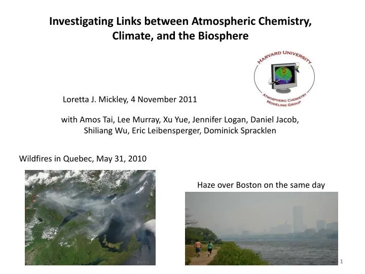
Investigating Links between Atmospheric Chemistry, Climate, and the Biosphere. Loretta J. Mickley, 4 November 2011. with Amos Tai, Lee Murray, Xu Yue , Jennifer Logan, Daniel Jacob, Shiliang Wu, Eric Leibensperger , Dominick Spracklen. Wildfires in Quebec, May 31, 2010.

E N D
Investigating Links between Atmospheric Chemistry, Climate, and the Biosphere Loretta J. Mickley, 4 November 2011 with Amos Tai, Lee Murray, XuYue, Jennifer Logan, Daniel Jacob, Shiliang Wu, Eric Leibensperger, Dominick Spracklen Wildfires in Quebec, May 31, 2010 Haze over Boston on the same day 1
Atmospheric chemistry examines the mix of gases and particles in the atmosphere. Our group mainly focuses on short-lived species: ozone, particles, mercury and their precursors, with lifetimes days to weeks. Lifetimes in atmospheric chemistry Centuries: SF6, some CFCs Decades: most greenhouse gases: CO2, N2O, . . . 9-10 years: CH4 (methane, precursor to ozone and greenhouse gas) Days-weeks: O3 (ozone), particulate matter (PM) Seconds: OH, NO Pollution over Hong Kong Air pollution over Hong Kong reached dangerous levels one of every eight days in 2009
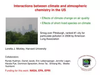
Surface ozone and particulate matter are harmful to human health. Number of people living in areas that exceed the national ambient air quality standards (NAAQS) in 2008. Calculated with standard of 0.075 ppm. Proposed new standards will push more areas into non-attainment. 2009 Short-lived species respond to climate change as well as to trends in emissions. EPA’s Technical Support Document for the proposed finding on CO2 as a pollutant. Cites the threat of climate change to air quality
Surface ozone and particulate matter also affect climate. Many particles scatter incoming sunlight (cooling). Ozone absorbs outgoing terrestrial radiation (warming) particles ozone visible infra- red IPCC 2007 Radiative forcing W m-2 Yardstick of warming or cooling effect
O2 Lifecycle of tropospheric ozone: production is viaoxidation of CO, VOCs, and methane in the presence of NOx. hn O3 STRATOSPHERE Many processes affected by climate 8-18 km TROPOSPHERE Soup of chemical reactions Ozone is produced in the atmosphere in sunlight. NOx O3 CH4 Deposition CO VOCs VOCs NOx NOx CO NOx VOCs NOx CH4 VOCs VOCs NOx emissions Biosphere Fires Human activity • Nonmethane volatile organic compounds (VOCs) • NOx = NO + NO2 5
1988, hottest on record Days Observations imply importance of biogenic emissions to atmospheric chemistry Probability of ozone exceedance • Reasons for increasing probability of ozone exceedances at higher max Temps: • Greater stagnation + clear skies • Faster chemical reactions. • Greater biogenic emissions, e.g. isoprene Northeast/ mid Atlantic in summer Probability maximum daily temperature (K) Number of summer days with ozone exceedances, mean over sites in Northeast Lin et al., 2000
. . . . . . Climate change affects many processes, including gas-particle partitioning. Life cycle of particulate matter (PM, aerosols) ultra-fine (<0.01 mm) fine (0.01-1 mm) cloud (1-100 mm) precursor gases nucleation cycling coagulation condensation Soup of chemical reactions coarse (1-10 mm) scavenging SO2 SO2 VOCs NOx NOx VOCs VOCs NOx NH3 VOCs NOx VOCs NOx combustion volcanoes agriculture biosphere soil dust sea salt wildfires combustion
particulate matter (PM) and ozone pollution emissions transport dilution chemistry population winds Winds carry pollutants to other boxes. Emissions + chemistry calculated within box Models are useful tools to interpret observations and to investigate past or future atmospheres. GEOS-Chem chemical transport model: Global 3-D model describes the transport and chemical evolution of atmospheric pollutants Meteorology driving GEOS-Chem can come from observations or climate models.
Meteorology driving 3-D chemical models comes from climate models: • Two ways to run climate models • “nudged” with observations • calculated from first principles • All climate models depend on basic physics to describe motions and thermodynamics of the atmosphere: • E.g., vertical structure is described by hydrostatic equation Climate models also depend on parameterizations for many processes. E.g., microphysics of cloud droplet formation. Output Climate model Input Physics + Parameterized processes Tilt of earth, geography, greenhouse gas content Weather + Climate
observations model Validation of models involves scrupulously comparing model results to observations. Since, 1800s, input of reactive nitrogen to ecosystems has increased by more than a factor of 3 globally due to human activity. r = Correlation coefficients NMB = normalized mean biases MNB= mean normalized biases Zhang et al., 2011 Nitrate wet deposition fluxes, 2006
Biogenic volatile organic compounds (BVOCs): Emissions Parameterization in GEOS-Chem INPUTS Base emission for a specified mix of different plant functional types at specified meteorological conditions MODEL Base emissions are scaled for local conditions: vegetation type, leaf area index, temperature, solar insolation OUTPUT Big isoprene emitters: Oaks, spruce, firs, sweetgum Gridded BVOC emissions [atoms C cm-2 s-1] (includes isoprene and monoterpenes) Guenther et al., 2006
Other parameterizations in GEOS-Chem Soil NOx emissions = f(vegetation type, temperature, precipitation history, canopy reduction, fertilizer usage) Dry deposition = Resistance in series scheme, with these resistances: Aerodynamic resistance to surface Boundary resistance at surface of leaf Canopy surface resistance = f(Leaf area index, direct and diffuse sunlight, gas or particle type) Wet deposition = f(clouds, rainfall, gas or particle type) Difficulty is scaling up from small-scale processes to global scale.
How will changing climate affect changing organic carbon particles in the atmosphere? Fine mass of organic particles, annual mean. Southeast is a big contributor due to dense vegetation. Organic particles contribute about 20-40% of particle mass in the US. What will change in future atmosphere: air temperature biogenic emissions land use vegetation Malm et al., 2004
Effects of Future Biosphere Changes on Air Quality Biogenic volatile organic compound (VOC) + + Secondary organic aerosol (SOA) Plants Simulated 2000-2100 changes in annual surface SOA concentrations climate change only climate-driven biogenic emissions change only anthropogenic land use change only [Heald et al. 2008]
Effects of Future Biosphere Changes on Air Quality Climate- and CO2-driven 2000-2100 changes in areal fractional coverage Temperate broad-leaved trees Boreal needle-leaved trees Associated changes in SOA concentrations 20% increase in SOA global burden [Wu et al. 2011]
Effects of Future Biosphere Changes on Air Quality - + Leaf surface Ozone loss Plants + - Ozone increase or loss (depends on NOx) Biogenic VOC + ppb Simulated 2000-2150 changes in surface ozone concentrations Ozone deposition could have consequences for carbon uptake in plants. climate- and CO2-driven vegetation change only [Wu et al. 2011] [Wu et al. 2011]
Increasing ozone due to climate change can decrease gross primary productivity. 2000 ozone 2100 ozone GPP GPP 2000-2100 changes gross primary productivity due to ozone changes Sitch et al., 2007
Observed Meteorology Observed Area burned Regression Model Relationship between area burned + meteorology How will changing climate affect wildfires and air quality? model observations We build a fire prediction scheme that can capture interannual variability in area burned in the Western US. Area burned = f (temperature, rainfall, Palmer drought index, relative humidity, other indices. . .) Each ecosystem has its own relationship between area burned and meteorology. Yue et al., 2011
Temperature Temperature DJF JJA Ensemble of climate models predict warmer and drier summers in the west. Precipitation Precipitation 2000-2050 change in meteorological fields, ensemble medians in each gridbox. A1B scenario – moderate increases in greenhouse gases. Relative Humidity Relative Humidity Yue et al., 2011
Meteorology from 15 climate models Regression Model Calculated area burned for present-day and future 2000-2050 changes in meteorology from 15 IPCC AR4 climate models. different ecosystems in Western US We calculate changes in area burned for 2000-2050, using an ensemble of IPCC model results. Area burned increases 20-120% across Western US, but models show range of uncertainty. Spracklen et al., 2009 Yue et al., 2011 20
1986 1990 1995 2000 2051 2055 2060 2065 Years Present-day observations Ensemble median values of predictions Spread of predictions 1990 2000 2055 2065 The total area burned is predicted to increase by 60~120% over western US by the midcentury 105 ha Change in area burned is especially large in Southwest US, where area burned doubles. 105 ha Yue et al., 2011
The length of fire season increases by 3 weeks in 2050s relative to present day. End day 163 days 185 days Start day Calculations with observations Ensemble median values of predictions Spread of predictions Yue et al., 2011
Can we also simulate the effects of insect outbreaks on forests in a global chemistry model? Both fires and insect outbreaks are influenced by climate. Can we build a probabilistic model of insect outbreaks by ecosystem? Arneth and Niinemets, 2010
Annual mean emissions of isoprene Present-day Preindustrial CLIMAP LGM Webb LGM Investigations of the oxidation capacity of the atmosphere during the Last Glacial Maximum Ongoing project to look at how changing land cover and climate affect oxidation capacity of atmosphere. Biogenic species could play a role: decreased concentrations could increase OH levels. Emissions of biogenic species Murray et al., in progress
1950 1960 1970 1980 1990 2001 Trend in aerosols over United States suggests cleaner skies, possible warming. Calculated trend in surface sulfate concentrations, 1950- 2001. Sequence shows increasing sulfate from 1950-1980, followed by a decline in recent years. Most of aerosol has already cleared by 2010. Comparison to observed sulfate concentrations shows good agreement. Leibensperger et al., 2011
We test the effect of changing U.S. aerosols on regional climate. Two scenarios. 1950 1975 2000 2025 2050 GISS GCM A1B greenhouse gases constant aerosols A1B greenhouse gases zero US aerosols Each scenario includes an ensemble of 3 simulations. Mickley et al., 2011
Removal of anthropogenic aerosols over US increases annual mean surface temperatures by 0.5 o C. Summertime temperatures increase as much as 2 oC during heatwaves. Warming due to 2010-2050 trend in greenhouse gases. Additional warming due to zeroing of US aerosols Mean 2010-2050 temperature difference: No-US-aerosol case – Control White areas signify no significant difference. Results from an ensemble of 3 for each case. Mickley et al., 2011
Calculation of maximum temperatures in climate models is sensitive to choice of parameters having to do with land cover/soil. Lower estimate Upper estimate Lower and upper estimates of JJA maximum temperatures in 2x CO2 atmosphere Central 80% range of increases for 44 versions of one climate model oC 0 8 Forest roughness parameter Vegetation root depth Percent variability in Tmax accounted for by vegetation parameters. 6% 30% 50% Clark et al., 2010
Effect of kudzu invasion on surface air quality By fixing atmospheric nitrogen at a rapid rate, kudzu invasion leads to significant release of nitric oxide, an ozone precursor. kudzu native NO days N2O Calculated change in the number of ozone exceedance days in summer due to a 28% increase in soil NOx emissions accompanying large kudzu invasion. Mean July emissions at 3 sites in Georgia Hickman et al., 2010
Collaborations with ecologists: • Enhance knowledge of interactions between biosphere and atmosphere, and how to model those interactions • Improve understanding of response of ecosystems to climate change • Specific processes that will change with changing climate or changing emissions • biogenic emissions, including methane, VOCs • deposition of nitrogen, ozone, and other species • soil NOxemissions • insect-driven outbreaks and their consequences