Download
1 / 24
240 likes | 352 Vues
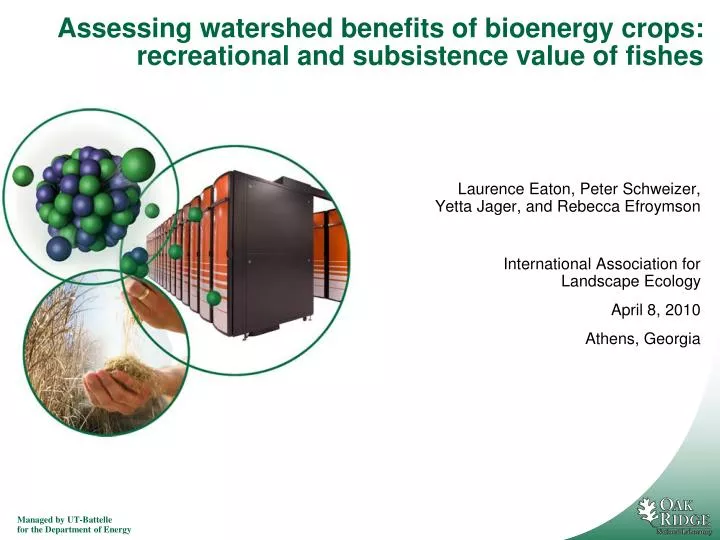
Assessing watershed benefits of bioenergy crops: recreational and subsistence value of fishes. Laurence Eaton, Peter Schweizer , Yetta Jager , and Rebecca Efroymson International Association for Landscape Ecology April 8, 2010 Athens, Georgia. Motivation.

E N D
Assessing watershed benefits of bioenergy crops: recreational and subsistence value of fishes Laurence Eaton, Peter Schweizer, YettaJager, and Rebecca Efroymson International Association for Landscape Ecology April 8, 2010 Athens, Georgia
Motivation • Could there be conflicting social and ecological objectives in increasing biomass production? • Why anglers? • Consume ecological and biophysical final goods • Promote economic development • Responsive to quality (richness) and quantity of fishing opportunities?
Presentation Outline • Overview • Approach and Data • Model • Results • Conclusion
Overview: Conceptual Framework • EISA mandates 21 billion gallons of second generation by 2022. • New landscapes include • Switchgrass and miscanthus • hybrid poplar, pine, eucalyptus, and willow (SRC) • Different landuse scenarios vary in association with water quality and aquatic biodiversity • Q: What is the relationship between fish richness and fishing privilege and activity?
Overview: POLYSYS modeling framework • Simulates US Agricultural Sector • Billion Ton Study Update ongoing • USDA baseline forecasts • County-level supply curves • Includes perennial crops, fixed land supply • Representative 2030 scenario: • $60/dt market price, perennial crop annual yield growth 4%
Overview: Resource Assessment and Agricultural Forecasting • Preliminary POLYSYS scenarios of biofuels market for perennial biomass crops production • Highest conversion to switchgrass is from wheat and pastureland
Overview: Approaches to ecological valuation • Total Value (market, non-market, surrogate) • Macro- top down • Environmental/Economic indicies • Micro- bottom up • “Travel Cost Method” (TCM) • “Contingent Valuation Method” (CVM) • Revealed Behavior approach Loomis, 2005
Approach: Economic Model • Total use = f (F, C, B) • Where • Total use= resident and non-resident activity days (based upon privilege status and total trip days) • F= ecological final goods (e. g. lakes, streams, rivers) • C= capital infrastructure (e. g. access to sites) • B= biophysical final goods (native fish richness and native game fish richness)
Data: Sources and method • County-level license sales (2008-9) • National Survey of Fishing, Hunting, and Wildlife-Associated Recreation (2006) • Net Economic Values of Wildlife-Related Recreation in 2006 (2009) • Total Privilege • Population with fishing rights • Temporary (6 classes,1 day - 2 weeks) • Annual (2 classes, annual fishing and combo) • Activity days • Income unobserved • Allows combining temporary and annual privileges, (Total and Nonresident activity days correlation .95, and Total and Resident activity correlation .99) Revealed Behavior Fishing Privilege
Approach: Study area and data Native Gamefish Richness • Arkansas White Red River Basin HUC-8 regions (n=173) • 8 states, 322 counties, 1353 census tracts, 7783 block groups (lowest level of census population reporting)
Approach: Data Arrangment County Level License Sales Information County-Level CENSUS Population Characteristics Block Group Level License Sales Block Group Level CENSUS Population Characteristics Dependent Variable + Fishing Activity State Level Activity Information (USFWS) State Level Activity Days and Expenditures Biophysical Final Goods by HUC Native fish Species by HUC 8 Boundary Nature Serve Native Fish Richness Explanatory Variables Native Game Species by HUC 8 Road Density Ecological Goods Stream lengths/Surface water Environmental Quality Attributes Sediment
Model: Full Linear Regression Total Use = f (Pop, N, G, S, A, Pw, Elev_Drain, TMDL, Stream2max, Stream3plus) • Where • Total Use= resident and nonresident privilege and activity days • Pop= total population by HUC • N = total native fish species • G = total native game fish species • S = sediment concentration (mg/kg) • A = road density • Pw = percent of surface water by HUC • Elev_Drain = elevation drainage • TMDL= Total Maximum Daily Limit • Stream2max = first and second order stream lengths • Stream3plus = length of streams at third and higher order • Estimated using a log-link Poisson distribution regression
Current Model Limitations Specification of stocked warm and cold water fishes (Loomis, 1998) Spatial resolution of fishery information Spatial context of population Quantitative fish density data Angling success and satisfaction
Results: Residual of observed and predicted activity days Spearman R= 0.816 (p<.0001); Pearson R= 0.753 (p<.0001)
Conclusion We combine socioeconomic and ecological parameters to predict direct use, with correct anticipated sign of coefficients Omitted variable bias could be due to error in estimating total population, recreational amenities, and stocking frequency and distribution Total valuation of fishes in this area is a much larger and complex process
Future research • Improving population estimates (raster approach) • Extending travel cost method to include driving distance to water • Multi-metric approach to ecosystem valuation related to fishes (including rare species; net economic value; non-use values; intrinsic values) • Forecast use changes from future landscape and water quality scenarios
Acknowledgements Latha Baskaran, Bob Perlack, Anthony Turhollow, Mark Downing (ORNL) Virginia Dale (CBES-ORNL) Chad Hellwinckel (UT-APAC) Oak Ridge Associate Universities (ORAU) ORISE Program
Public Perceptions “With the 1980s and the rise of the Conservation Reserve Program, the Driftless Area's prairie character began to re-emerge. Today 33 trout streams in the area support natural spawning…. But now anglers worry that high corn prices caused by demand for ethanol could erase those gains, as more lands are put back to agricultural use.”