Download
1 / 28
280 likes | 288 Vues
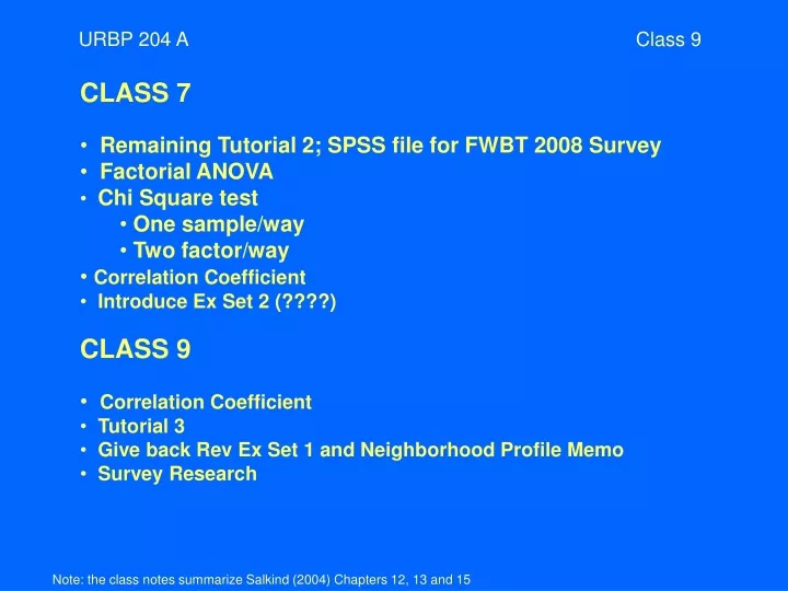
URBP 204 A Class 9. CLASS 7 Remaining Tutorial 2; SPSS file for FWBT 2008 Survey Factorial ANOVA Chi Square test One sample/way Two factor/way Correlation Coefficient Introduce Ex Set 2 (????). CLASS 9 Correlation Coefficient Tutorial 3

E N D
URBP 204 A Class 9 • CLASS 7 • Remaining Tutorial 2; SPSS file for FWBT 2008 Survey • Factorial ANOVA • Chi Square test • One sample/way • Two factor/way • Correlation Coefficient • Introduce Ex Set 2 (????) • CLASS 9 • Correlation Coefficient • Tutorial 3 • Give back Rev Ex Set 1 and Neighborhood Profile Memo • Survey Research Note: the class notes summarize Salkind (2004) Chapters 12, 13 and 15
Correlation How the value of one variable changes if the value of the other variable changes. For example, correlation between: Distance from city center and housing price Both variables need to be ratio or interval level. Note: the class notes summarize Salkind (2004) Chapters 12, 13 and 15
Correlation Coefficient Q: How do we know of the correlation is statistically significant? A: Test for significance of the correlation coefficient Source: Salkind, p 230 Note: the class notes summarize Salkind (2004) Chapters 12, 13 and 15
Steps for testing 1. Statement of null and research hypothesis H0: ρxy = 0 No relationship between variables x and y H1: rxy = 0 There is relationship between variables. 2. Set level of risk Level of risk of type I error = 5%, or level of significance = 0.05 3. Selection of appropriate test statistic Choose t-test for the significance of the correlation coefficient Note: the class notes summarize Salkind (2004) Chapters 12, 13 and 15
Coefficient of correlation 4. Obtained value For relationship between Density and distance , r = - 0.74 Density and price, r = 0.81 Distance and price, r = - 0.98 Note: the class notes summarize Salkind (2004) Chapters 12, 13 and 15
5. Determination of the value needed for rejection of null hypothesis (critical value) See table B4, pg. 365 Critical value = 0. 35 (see Salkind, p.363) 6. Comparison of obtained and critical value Obtained value more extreme than the critical value for following relationships: Density and distance , r = - 0.74 Density and price, r = 0.81 Distance and price, r = - 0.98 7. Decision Reject the null hypothesis (null hypothesis - there is NO relationship between the variables). The relationship is not due to chance alone. Degree of freedom = n-2 = 30-2 = 28 Note: the class notes summarize Salkind (2004) Chapters 12, 13 and 15
Non parametric tests • When assumption of normality does not hold (small sample size – less than 30 observations) • Need ordinal or nominal level data. Note: the class notes summarize Salkind (2004) Chapters 12, 13 and 15
One factor/sample chi square Is the distribution of frequencies what you would expect by chance alone? 1. Statement of null and research hypothesis Proportion of occurrence under each category is equal. H1: Proportion of occurrence under each category is not equal. 2. Set level of risk Level of risk of type I error = 5%, or level of significance = 0.05 3. Selection of appropriate test statistic Choose chi square test H0: P1 = P2 = P3 = P4 = P5 P1 = P2 = P3 = P4 = P5
4. Obtained value Note: Should have minimum of 5 observations under each category Note: the class notes summarize Salkind (2004) Chapters 12, 13 and 15
5. Determination of the value needed for rejection of null hypothesis (critical value) See table B5, pg. 367 Critical value = 9.49 (see Salkind, p.363) 6. Comparison of obtained and critical value Obtained value more extreme than the critical value 7. Decision Reject the null hypothesis (null hypothesis - that the distribution of frequencies is equal). Degrees of freedom = number of categories of data – 1 = 5-1 = 4
Two factor/way chi square Explore relationships when both the dependent and the independent variables are nominal or ordinal level, that is “Categorical data” Does the respondents’ age affect their perception about the condition of street lighting? 1. Statement of null and research hypothesis Proportion of occurrence under each category is equal. H1: Proportion of occurrence under each category is not equal. 2. Set level of risk Level of risk of type I error = 5%, or level of significance = 0.05 3. Selection of appropriate test statistic Choose chi square test H0: P1 = P2 = P3 = P4 P1 = P2 = P3 = P4
4. Obtained value Note: Should have minimum of 5 observations under each category Expected Frequency Table Observed Frequency Table 9.75 = (26 x 15) / 40 16.25 = (26 x 25) / 40 5.25 = (14 x 15) / 40 8.75 = (14 x 25) / 40 λ2 = (6-9.75)2 / 9.75 + (20-16.25)2 /16.25 + (5.25-9)2 /5.25 + (8.75-5)2 /8.75 = 6.59
URBP 204 A Class 6 5. Determination of the value needed for rejection of null hypothesis (critical value) See table B5, pg. 367 Critical value = 3.84 (see Salkind, p.363) 6. Comparison of obtained and critical value Obtained value more extreme than the critical value 7. Decision Reject the null hypothesis (null hypothesis - that the distribution of frequencies is equal). Degrees of freedom = (row-1) x (column -1) = (2-1) x (2-1) = 1 x 1 = 1
Sampling Because we can not survey the entire population, hence we survey a smaller proportion of the population, that is, the sample. The methodology of choosing the sample - sampling Desired characteristic of the sample - representativeness Probability Sampling Non probability Sampling - Reliance on available subjects - Purposive/ judgmental - Snowball - Quota sampling - Selecting informants Note: the class notes summarize Babbie (2004) Chapter 7, and part of Chapter 9.
Non- Probability Sampling • Reliance on available subjects • Stopping people at street corner • In-class survey • Purposive / Judgmental Sampling • Selecting a sample on the basis of prior knowledge • Study only selected single-family residential or multi-family houses • because you already know that they are representative of the entire • population • Study of deviant cases • Snowball Sampling • - Identify few subjects and use their help in identifying other subjects • e.g. homeless; drug users, etc. Note: the class notes summarize Babbie (2004) Chapter 7, and part of Chapter 9.
Non- Probability Sampling contd…. • Quota Sampling • - Classify the target population based on its characteristics • Assign weights and numbers to survey on the basis of proportion • Choice of respondents within the classification may not be random • Selecting Informants • - The informant talks about the group – s/he represents the group • - Study of cults; neighborhood organization • - Informant must truly “represent” the target group Note: the class notes summarize Babbie (2004) Chapter 7, and part of Chapter 9.
Probability Sampling • All members of the population should have equal chance of being selected • Why? To remove bias – time of day; kinds of people; socio- economic status, etc. etc. • Some definitions: • Element - e.g. household; analogous to unit of analysis in data analysis • Population – aggregation of all elements that can be theoretically possible in a study- e.g. all households in FWBT area • Study population - actual population from which the sample is selected Note: the class notes summarize Babbie (2004) Chapter 7, and part of Chapter 9.
Probability Sampling Why do we need probability theory in sampling? We need to be sure that the sample is representative of the population. For example: Neighborhood of 10,000 household Want to find the median h.h. income We take the sample of 100 h.h.s Population Parameter - median h.h. income of theneighborhood Statistic - median h.h. income of sample of 100 h.h.s Aim:Statistic is as close as possible to the populationparameter. That is, minimize the error due to sampling (sampling error) Note: the class notes summarize Babbie (2004) Chapter 7, and part of Chapter 9.
Probability Sampling Sampling distribution: normal curve! Sampling error Magnitude of the Sampling error depends upon: The parameter Sample size Standard Error How to Calculate Standard Error Population parameter: 50% bike and 50% do not. Sample size = 100 Standard error = 0.5 x 0.5 = 0.05 = 5% 100 Probability Theory indicates that: 68% of the sample statistics will fall within 1 std. error of the population parameter. 95% will fall within 2 standard errors 99.9% will fall within 3 standard errors In general: Standard error of the mean = s n Where s = standard deviation n= number of observations Note: the class notes summarize Babbie (2004) Chapter 7, and part of Chapter 9.
Sampling Distribution contd… • In reality: • we take only 1 sample, not a large number of them. • we only know the sample statistic, not the population • parameter! • But we know that 68% of the sample statistics fall within 1 standard • error, 95% within 2 standard errors, and 99.9% within 3 standard • errors. • Hence we can argue that we are 68% confident that any given • sample statistic will fall within 1 standard error of the population • parameter. • We replace population parameter with sample statistic to find standard • error • Confidence level = 68%; Confidence interval = 1 standard error • Confidence interval = 95%; Confidence interval = 2 standard error Note: the class notes summarize Babbie (2004) Chapter 7, and part of Chapter 9.
Types of probability sampling designs Simple random sampling All elements are numbered and then a predetermined number are randomly selected. (may get clusters, should know the entire population) Systematic sampling Every kth element chosen For e.g.: every 10th house; danger of biases (every 10th house may be a corner house - traffic noise) Stratified Sampling Reduce sampling error by less variability e.g. single-family houses and apartments Within the strata we may employ simple random or systematic sampling Multistage clustering sampling Sampling of clusters City-wide study - list census tracts - choose sample of census tracts - list all block groups - choose sample of block groups - list all blocks - choose sample of blocks - list all h.h.s - choose sample of h.h.s May also stratify the sample: Stratification in multistage cluster sampling Note: the class notes summarize Babbie (2004) Chapter 7, and part of Chapter 9.
Survey Research • Guidelines for asking questions • Open ended vs close ended question • Open ended – more rich; coding difficult; more chances of error while recording • Close ended – less rich; responses may be straight jacketed; less chances of recording • error; careful about exhaustiveness • Make items clear - income last year – based on W-2? • Avoid double-barreled questions – Should San Jose cut back on road • construction and increase allocation for affordable housing? • Respondent must be competent and willing to answer • Questions should be relevant • Keep it short Note: the class notes summarize Babbie (2004) Chapter 7, and part of Chapter 9.
Guidelines for asking questions contd…. • Avoid negative terms – do you think we should not do this? • Avoid biased items and terms – do you agree with the recent health reports’ finding that…… Note: the class notes summarize Babbie (2004) Chapter 7, and part of Chapter 9.
Guidelines for survey interviewing • Modest yet neat appearance • Avoid voice inflections • Be neutral • Be polite • Be familiar with the questions • Don’t add your words to the question • Record responses exactly • Gently probe for responses/ clarifications Note: the class notes summarize Babbie (2004) Chapter 7, and part of Chapter 9.
Questionnaire Construction • Not cluttered • Professional look; clear instructions on how to choose responses (especially if self-administered), • Use of contingency questions • Use of matrix format • Order of questions – bias due to the order (negative aspects of sprawl; then ask is sprawl bad); in self- administered begin with interesting questions; in interviews – uncomplicated questions first • Include clear instructions and introductory statements (now think about the last one week….) • Pretest the questionnaire
Self- administered Questionnaire Mail; home delivery or combination; questionnaire at a public gathering; etc. If mail delivery Monitor the return Follow up mailings Telephone Surveys Unlisted number – random digit dialing Advantages – cheap and quick; no dress code; probe more sensitive areas; more quality control possible as central location; safety. Disadvantages – compete with bogus surveys; easy to hang up; answering machines; cell phones
Comparison of self-administered and interview survey methods • Advantages of self- administered over face-to-face interviews • Cheaper • More geographically extensive • Require smaller staff • Easy to probe sensitive topics • Advantages of face-to-face interviews over self- administered questionnaires • Larger response rate • More effective for complicated issues • May also note other information - condition of the neighborhood, etc.
Strengths and weaknesses of survey research • Strengths • Describe characteristics of a large population • Make large samples feasible • More flexible – can cover several topics • Strong on reliability • Weakness • Have to ascribe the same intent to responses to questions related to complex concepts • Least common denominator – superficial in coverage of complex topics • Life situation/ context not known • Can not change questions mid-way • Respondent may form opinion at the moment • Weak on validity