Download
1 / 70
730 likes | 946 Vues
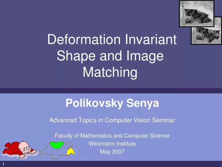
Deformation Invariant Shape and Image Matching. Polikovsky Senya Advanced Topics in Computer Vision Seminar Faculty of Mathematics and Computer Science Weizmann Institute May 2007. Based on…. Integral Invariants for Shape Matching

E N D
Deformation Invariant Shape and Image Matching Polikovsky Senya Advanced Topics in Computer Vision Seminar Faculty of Mathematics and Computer Science Weizmann Institute May 2007
Based on… Integral Invariants for Shape Matching Siddharth Manay, Daniel Cremers, Member, Byung-Woo Hong,Anthony J. Yezzi Jr., and Stefano Soatto Deformation Invariant Image Matching Haibin Ling ,David W. Jacobs
Part I : Invariant Shape Matching Can you guess what it is ?
Outline Integral Shape Matching • Introduction • Basic Definitions, Previous Work • Curvature • Integral Invariant (II) • Relation of Local Area II to Curvature • Shape Matching and Distance • Multi-scale Shape Matching • Implementation and Experimental Results
Applications of shape matching • Airport security : • Industry quality control : • Medical images analyses :
Ultimate Goal Compare objects represented as closed planar contours.
Basic Definition • Object : • Closed planar contour. • No self-intersections. • Shape : • Equivalence class of objects. Obtained under the action of a finite-dimensional group : Euclidean, similarity, affine, projective group.
Basic Definition (cont.) Two objects have the same shape if and only if one can be generated by transformation group actions on other shape. In Addition: - articulated - occluded - jagged (not obtained with standard additive, zero mean)
Summary Goal • Define a distance so that shapes that vary by Euclidean transformations have zero distance. • Shapes vary by scaling , articulation , occlusion have small distance. • Resistant to : “small deformations” “high-frequency noise” “localized changes”
Summary Goal (cont.) The babies should have low distance to each other, but high distance to other classes of shapes. Low distance High distance
Previous Work • Statistical approach using moments. [35],[27] High-order moments sensitive to noise. • Normalized Fourier descriptors. [93],[52],[2] High order Fourier coefficients are not stable with respect to noise. • Local neighborhoods using Wavelet transform. [83],[34]
Previous Work (Cont.) • Global radial histogram of the relative coordinates of the rest of the shape at each point. [6] • Differential invariants (Curvature) [44], [36], [17], [58], [76], [30], [48], [64], [91], [85], [37] 12
Curvature • Intuitively, curvature is the amount by which a geometric object deviates from being flat. Less general y = f(x) Plane curve c(t) = (x(t),y(t))
Curvature (cont.) • Curvature can be also be geometrical understood as in terms of osculating (kiss) circle and radius curvature. • Circle of radius r has curvature • 1/r everywhere . • Straight line r = ∞ has • curvature 1/ ∞ =0 everywhere • Features: • Invariant to rotation, reflections of the original curve. • NOT invariant to scaling.
Outline Integral Shape Matching Introduction Basic Definitions, Previous Work Curvature Integral Invariant (II) Relation of Local Area II to Curvature Shape Matching and Distance Multi-scale Shape Matching Implementation and Experimental Results
Integral Invariant • Closed planar contour. C:S1 → R2. ds - infinitesimal arclength. • G - transformation group acting on R2. dx - area %on R2. • μ curve C corresponding measure dμ(x).
Integral Invariant • Function I: R2 → R G-invariant if satisfies: • I(.) is associates to each point on contour a real number.
Step 1: Curvature Curvature κ(C) of curve C is G-invariant.
General notion of Integral Invariant • Function IC(p) : R2 →R is and integral G-invariant • Kernel k : R2 X R2 → R. • K( ● , ● ) : • p don’t necessarily lie on the curve C. p
Step 2: Distance integral invariant Unlike curvature distance invariant is R+. (Euclidean distance is always nonnegative) • For global descriptor , local change of a shape affects the values of the distance integral invariant for the entire shape.
Step 3: “Shape Context” Preserves locality can be obtained by weighting the integral with a kernel q(p, x). Local radial histogram.
Step 3: “Shape Context” (cont.) • NOT discriminative, same value for different geometric • features.
Finale Step: Local Area Integral Invar. • Define a ball Br(p), Br : R2 X R2 {0,1} ; ( R+ ) r – radius. p - center of the ball. C - interior of the region bounded by C.
Local Area Integral Invar.(cont.) r r • Naturally forms a multi-scale invariant.
Relation of Local AII to Curvature r r θ R C C • Assume that C is smooth curve, because of the curvature.
Outline Integral Shape Matching Introduction Basic Definitions, Previous Work Curvature Integral Invariant (II) Relation of Local Area II to Curvature Shape Matching and Distance Multi-scale Shape Matching Implementation and Experimental Results
Shape Matching and Distance • Shape distance is a scalar value that quantifies similarity of the two contours. D(C1,C2). • Basing on group invariant , integral invariant : • invariant to G group action. • robust to noise and local deformations • Corresponding points. C1 = C2= , Local Are Integral Invariant : I1 , I2
Corresponding points • Disparity function d(s). Reparameterizes C1 ,I1 and C2 ,I2 . • optimal point correspondence ( ~ denotes correspondence)
Energy Functional E(...,d) E1 - measures the similarity of two curves. E2 - elastic energy. α - control parameter α > 0. • If d(s) = 0 , direct match. • If d’(s) = 0 , circular “shifts”. • Other d(s), “stretch” , “shrink”.
Control Parameter α small α : d*(s) large α : d*(s)
Multi-scale Shape Matching Curvature Scale-space Integral Invariant Scale-space Trace of local extrema across scales Curvature scale-space is derived from Gaussian smoothing.
Multi-scale Shape Matching (cont.) • Matching shapes of different sizes. R R’ • Normalized kernel radius : r / R.
Multi-scale Shape Matching (cont.) Correspondences between two signals influenced by: Control parameter α. Size of the kernel width r. fine scale intermediate scale coarse scale
Outline Integral Shape Matching Introduction Basic Definitions, Previous Work Curvature Integral Invariant (II) Relation of Local Area II to Curvature Shape Matching and Distance Multi-scale Shape Matching Implementation and Experimental Results
Implementation Minimization of the energy functional E. C1[i+1] C1[i] v[I + 1, j + 1] v[i , j+1] v[i , j + 1] v[I + 1, j + 1] e e v[i , j] C1 v[i + 1, j] e v[i , j] v[i +1, j] C2[j+1] C2[j] e = v(i,j) → v(k,l) C2 Each point in each curve must have at least one corresponding point in the other curve.
Implementation (cont.) • Minimization of the energy functional E is equivalent to finding a shortest path that gives a minimum weight. v[I + 1, j + 1] v[i , j+1] e M 1 e C1 0 e C2 N 1 v[i +1, j] 0 v[i , j] nodes = MN edges = 3MN w(p) ← E(I1,I2,d) Graph used to compute the correspondence for two curves with M = N = 5.
Implementation (cont.) • In previous implementations we choose start point in C1and run all over C2. • Alternately, observing strong features, in the invariant space.
Experimental Results higher dissimilarity dissimilarity The gray levels indicate the dissimilarity between points lighter shade indicates higher dissimilarity.
Experimental Results (cont.) • 100 sample on contours • r = 15 • α = 0.1 “On Aligning Curves” [76]
Experimental Results (cont.) Curvature Int.Inv. Curvature Int.Inv. Curvature Histograms of shape distance between Shape 24 and 1,000 perturbations of Shape 20 with noise at variance = 2.5.
Experimental Results (cont.) higher dissimilarity dissimilarity Noisy shapes (across top) and original shapes (along left side) vie differential invariant
Experimental Results (cont.) higher dissimilarity dissimilarity Noisy shapes (across top) and original shapes (along left side) viaintegral invariant
Summary Curvature. Four Steps : • Curvature, sensitivity to noise. • Global descriptor, local change. • Local radial histogram, NOT discriminative. • Local Area Integral Invar. Shape Matching ,Multi-scale Shape Matching. Implementation. Results. M 1 0 C1 C2 N 1 0
Outline Introduction Deformation Invariant Framework Experiments Summary
General Deformation • One-to-one, continuous mapping. • Intensity values are deformation invariant. • (their positions may change) • Affine model for lighting change. (Out of the scope)
Solution • A deformation invariant framework • Embed images as surfaces in 3D • Geodesic distance is made deformation invariant by adjusting an embedding parameter • Build deformation invariant descriptors using geodesic distances
Outline Introduction Deformation Invariant Framework - Intuition through 1D images - 2D images Experiments Summary
1D Image Embedding 1D Image I(x): EMBEDDING I(x) ( (1-α)x, αI ) (1-α)x αI 2D Surface : Aspect weight α: measures the importance of the intensity