Download
1 / 40
410 likes | 614 Vues
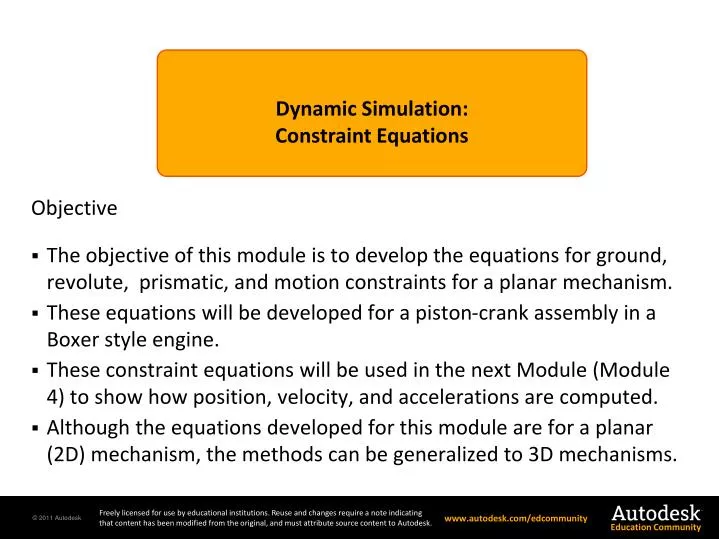
Dynamic Simulation : Constraint Equations. Objective The objective of this module is to develop the equations for ground, revolute, prismatic, and motion constraints for a planar mechanism. These equations will be developed for a piston-crank assembly in a Boxer style engine.

E N D
Dynamic Simulation: • Constraint Equations Objective • The objective of this module is to develop the equations for ground, revolute, prismatic, and motion constraints for a planar mechanism. • These equations will be developed for a piston-crank assembly in a Boxer style engine. • These constraint equations will be used in the next Module (Module 4) to show how position, velocity, and accelerations are computed. • Although the equations developed for this module are for a planar (2D) mechanism, the methods can be generalized to 3D mechanisms.
Boxer Style Engine Section 4 – Dynamic Simulation Module 3 – Constraint Equations Page 2 • Boxer style engines have a horizontally opposed piston configuration. • This has several advantages • Lower center of gravity • Lower vertical height • Lighter weight • Less vibration • Boxer style engines are used by Porsche and Subaru. • Because of their low vertical profile they are often called pancake engines.
Cross Section View Section 4 – Dynamic Simulation Module 3 – Constraint Equations Page 3 This module will use the piston-crank portion of this engine to demonstrate how kinematic and motion constraints are developed. Counterweight Rod Bolt Bottom Bearing Cap Cylinder Liner Piston Pin Bearing Piston Connecting Rod Piston Pin Crank Shaft Crank Bearing
Planar System Section 4 – Dynamic Simulation Module 3 – Constraint Equations Page 4 • The boxer engine rotating assembly contains four piston assemblies. • Constraint equations will be written for one piston assembly to demonstrate the process. • This single assembly can be represented as a planar mechanism. • A Dynamic Simulation of the complete system will be presented in another module. Cylinder 1 Cylinder 2 Cylinder 3 Cylinder 4 The planar equations will be developed for Cylinder 3.
Global Coordinate System Section 4 – Dynamic Simulation Module 3 – Constraint Equations Page 5 Z • The constraint equations will be referenced to the stationary coordinate system shown in the figure. • This reference coordinate system is called the global coordinate system. • Capital letters are used to indicate that a coordinate or vector refers to this coordinate system. • Lower case letters will be used to indicate a coordinate or vector is referred to a body fixed coordinate system associated with a part. X Cylinder 3 Y X
Part ID’s Section 4 – Dynamic Simulation Module 3 – Constraint Equations Page 6 The process of developing the constraint equations is facilitated by identifying each component by a letter. The five components shown with letters make up the basic system for which the constraint equations will be written. A Cylinder Liner E Crank Bearing (Not Visible) B Piston C Connecting Rod D Crank Shaft
Mobility Section 4 – Dynamic Simulation Module 3 – Constraint Equations Page 7 • Gruebler’s equation can be used to establish the mobility of the planar mechanism. • Bodies (B) = 5 • Grounded bodies (G) = 2 • Revolute joints (R) = 3 • Prismatic joints (P) = 1 A Cylinder Liner E Crank Bearing (Not Visible) Mobility B Piston C Connecting Rod A mobility of one will require one motion constraint. D Crank Shaft
List of DOF’s Section 4 – Dynamic Simulation Module 3 – Constraint Equations Page 8 • The DOF’s are associated with a set of generalized coordinates. • Each body has 3 DOF and 3 generalized coordinates. • The generalized coordinates for the planar mechanism are listed on the right. • Fifteen constraint equations must be developed that will enable each of the fifteen generalized coordinates to be determined. List of Generalized Coordinates Format X-coordinate of the cg of Body A Body Capital letter indicates that variable is associated with the global coordinate system. Center of Gravity
Section 4 – Dynamic Simulation Module 3 – Constraint Equations Page 9 • The cylinder liners are pressed into the engine block and do not move. • The pistons move relative to the cylinder liners and the combination make a prismatic joint. • The cylinder liners must be mathematically grounded or fixed in space. Cylinder 1 Cylinder 2 Ground Joints Cylinder 3 Cylinder 4
Cylinder Liner Ground Equations Section 4 – Dynamic Simulation Module 3 – Constraint Equations Page 10 The location of the center of gravity and the orientation of the principal axes of inertia are shown in the figures. The ground constraint equations that fix the position of the c.g. and orientation of the principal axes can be written as y x y z
Crank Bearing Ground Joint Section 4 – Dynamic Simulation Module 3 – Constraint Equations Page 11 Virtual Crank Bearing Located at the Origin • The crank bearing is fixed in the engine block and does not move. • The crank shaft rotation relative to the crank bearing can be represented by a revolute joint. • All of the parts in the planar system must lie in the global X-Y plane. • Therefore, a “virtual” crank bearing will be placed at the origin of the global coordinate system so that the planar equations can be developed. Y Z X Crank Bearing Constraint Equations
Summary of Ground Joint Equations Section 4 – Dynamic Simulation Module 3 – Constraint Equations Page 12 Cylinder Liner Virtual Crank Bearing • Each of these equations fix one DOF for the respective part in space. • None of the equations are a function of time. • None of the equations involve more than one part.
2D Coordinate Transformation Matrix Section 4 – Dynamic Simulation Module 3 – Constraint Equations Page 13 • In subsequent slides it will be necessary to transform the components of a vector from a body fixed coordinate system to the global coordinate system. • This transformation is accomplished with the transformation matrix [T(q)]. • From the figure, Y x y X Matrix Form
Revolute Joint Section 4 – Dynamic Simulation Module 3 – Constraint Equations Page 14 yB • There are three revolute joints in the piston-crank assembly • Between the piston and connecting rod • Between the connecting rod and crankshaft • Between the crankshaft and crank bearing • The constraint equations for a revolute joint will be developed using the two bodies shown in the figure. • Body A and B have the same translational motion at the joint but can have relative rotation. Body B Y xB Body A qB yA xA Joint qA X Two bodies connected at a common point that allows relative rotational motion.
Revolute Joint Section 4 – Dynamic Simulation Module 3 – Constraint Equations Page 15 • The position of Joint 1 on Body A relative to the global coordinate system is given by the equation • The components of are written with respect to the global coordinate system base vectors and the components of are written with respect to the body fixed coordinate system. Y Joint 1 yA Body A 1 xA qA X
Revolute Joint Section 4 – Dynamic Simulation Module 3 – Constraint Equations Page 16 • The components of the body fixed position vector must be transformed to the global coordinate system before the components of the two vectors can be added. • This is accomplished using the transformation matrix introduced earlier. Position Vector Equation Component Form
Revolute Joint Section 4 – Dynamic Simulation Module 3 – Constraint Equations Page 17 • In a Revolute Joint the coordinates of the joint must be same for each body. • Thus, • The coordinates of Joint 1 on Body A are • Similarly, the coordinates of Joint 1 on Body B are or General Form of the Constraint Equations for a Planar Revolute Joint
Revolute Joint Section 4 – Dynamic Simulation Module 3 – Constraint Equations Page 18 • The general form of the constraint equations for a planar revolute joint is • The specific equations for the three revolute joints in the piston-crank mechanism will now be developed Joint 1 2nd Revolute Joint Joint 2 Joint 3
1st Revolute Joint Section 4 – Dynamic Simulation Module 3 – Constraint Equations Page 19 Piston Body B • The location of the joint relative to the c.g. is needed to define the parameters & • For the piston, 28 mm y x C.G. Joint 1
1st Revolute Joint Section 4 – Dynamic Simulation Module 3 – Constraint Equations Page 20 • The location of the joint relative to the c.g. is needed to define the parameters & • From the picture, Connecting Rod Body C 102.6 y x Joint 1
1st Revolute Joint Section 4 – Dynamic Simulation Module 3 – Constraint Equations Page 21 Using the geometry from the piston and connecting rod, the revolute joint constraint equation becomes Joint 1 1st Revolute Joint Constraint Equations
2nd Revolute Joint Section 4 – Dynamic Simulation Module 3 – Constraint Equations Page 22 General Form of Constraint Equation • The location of the joint relative to the c.g. is needed to define the parameters & • From the picture, Body C y Joint 2 x 41.3 mm
2nd Revolute Joint Section 4 – Dynamic Simulation Module 3 – Constraint Equations Page 23 General Form of Constraint Equation • The location of the joint relative to the c.g. is needed to define the parameters & • From the picture, y x Joint 2 43 mm
2nd Revolute Joint Section 4 – Dynamic Simulation Module 3 – Constraint Equations Page 24 Using the geometry from the connecting rod and crank shaft, the revolute joint constraint equation becomes Joint 2 2nd Revolute Joint Constraint Equations
3rd Revolute Joint Section 4 – Dynamic Simulation Module 3 – Constraint Equations Page 25 General Form of Constraint Equation • The c.g.’s of both the crank and crank shaft lie at the origin of the global coordinate system. • Therefore, the body fixed coordinates of the joint relative to the c.g. are zero. Joint 3 3rd Revolute Joint Constraint Equations
Summary of Revolute Joint Equations Section 4 – Dynamic Simulation Module 3 – Constraint Equations Page 26 Body C Body B Body C 2nd Revolute Joint Body D Joint 2 Joint 1 Joint 3 Body E Body D
Prismatic Joint Section 4 – Dynamic Simulation Module 3 – Constraint Equations Page 27 yA • In the planar system the cylindrical joint between the cylinder liner and the piston acts like a prismatic joint. • A prismatic joint allows two bodies to translate relative to each other along a common axis. • The two bodies cannot rotate independent of each other. • The equations for a planar prismatic joint are based on the geometry shown in the figure. Y Common Axis Body B Body A yA xA qB xA qA X Two bodies A & B that translate relative to one another along a common axis.
Prismatic Joint Constraint Equations Section 4 – Dynamic Simulation Module 3 – Constraint Equations Page 28 • The points P and Q in Body A lie on the common axis and are connected by the vector PQ. • The points R and S in Body B lie on the common axis and are connected by the vector RS. • The vector PR also lies on the common axis and connects the points P and R. • The three vectors must be parallel. • Alternatively, vectors PR and RS must be perpendicular to . yA Y Common Axis Body B S R Body A yA xA Q qB xA P qA X Two bodies A & B that translate relative to one another along a common axis.
Prismatic Joint Constraint Equations Section 4 – Dynamic Simulation Module 3 – Constraint Equations Page 29 yA • The vector PQ with components written with respect to the body fixed coordinate system of Body A are • The components of the vector PQ with respect to the global coordinate system are Y Body B S R Body A yA xA Q qB xA P qA X Two bodies A & B that translate relative to one another along a common axis.
Prismatic Joint Constraint Equations Section 4 – Dynamic Simulation Module 3 – Constraint Equations Page 30 • The vector RS with components written with respect to the body fixed coordinate system of Body B are • The components of the vector RS with respect to the global coordinate system are yA Y Body B S R Body A yA xA Q qB xA P qA X Two bodies A & B that translate relative to one another along a common axis.
Prismatic Joint Constraint Equations Section 4 – Dynamic Simulation Module 3 – Constraint Equations Page 31 • The third vector is directed from point P to point R. • Point P has the coordinates • Point R has the coordinates • The vector has components yA Y Body B S R Body A yA xA Q qB xA P qA X Two bodies A & B that translate relative to one another along a common axis.
Prismatic Joint Constraint Equations Section 4 – Dynamic Simulation Module 3 – Constraint Equations Page 32 yA • The vector perpendicular to PQ has components • The dot product of two vectors that are perpendicular to each other is zero. Y Body B S R Body A yA xA Q qB xA P qA X First Constraint Eq. Two bodies A & B that translate relative to one another along a common axis. Second Constraint Eq.
Prismatic Joint Constraint Equations Section 4 – Dynamic Simulation Module 3 – Constraint Equations Page 33 • Substituting the vector components from the previous slides into the first constraint equation yields • Substituting the vector components from the previous slides into the second constraint equation yields
Summary of Prismatic Constraint Equations Section 4 – Dynamic Simulation Module 3 – Constraint Equations Page 34 The two constraint equations for a planar prismatic joint are 1st Constraint Equation 2nd Constraint Equation The vector components at the beginning and end of each equation are based on the body fixed coordinate systems and are constant. The only variables are the generalized coordinates of Body A and B. These equations are easily evaluated in a computer program.
Prismatic Joint Section 4 – Dynamic Simulation Module 3 – Constraint Equations Page 35 • The prismatic joint formed by the cylinder liner and the piston lies along the global X-axis. • Point P is chosen to lie at the c.g. of the cylinder liner. • Point Q is chosen to lie 1 mm to the right on the x-axis. • Point R is chosen to lie at the c.g. of the piston. • Point S is chosen to lie 1 mm to the right on the x-axis. y y x x P Q R S Vector components of PQ Vector components of RS Point Coordinates
Prismatic Joint Section 4 – Dynamic Simulation Module 3 – Constraint Equations Page 36 Substitution of the vector components and point coordinates into the two prismatic joint equations yields 1st Constraint Equation which reduces to 2nd Constraint Equation
Motion Constraint Section 4 – Dynamic Simulation Module 3 – Constraint Equations Page 37 • One motion constraint is required to make the mechanism stable. • The rotation of the crankshaft (Body D) will be given an angular speed of 3,000 rpm. • A 3,000 rpm engine speed is equal to 314 rad/sec. • Although all fifteen generalized coordinates are a function of time, this is the only constraint equation that explicitly contains time as a variable. Motion Constraint
Summary of Constraint Equations Section 4 – Dynamic Simulation Module 3 – Constraint Equations Page 38 There are five planar bodies each having three DOF giving a total of fifteen DOF. Fifteen unknowns requires fifteen equations. Revolute Joint 3 Revolute Joint 1 Ground Constraint 1 Revolute Joint 2 Motion Constraint Ground Constraint 2 Prismatic Joint
Summary of Constraint Equations Section 4 – Dynamic Simulation Module 3 – Constraint Equations Page 39 • Only one of the constraint equations is time dependent (Motion Constraint). • Most of the constraint equations are non-linear. • All of the constraints are algebraic equations and none are differential equations. • Geometric quantities (dimensions and distances) contained in the constraint equations can be found from information in a 3D CAD model.
Module Summary Section 4 – Dynamic Simulation Module 3 – Constraint Equations Page 40 • The constraint equations for ground, revolute, and prismatic joints have been developed for a planar mechanism. • The constraint equation for a rotational motion constraint has been developed for a planar mechanism. • These equations were used to determine the fifteen equations necessary for a piston-crank assembly taken from a Boxer engine model. • In some cases the constraint equations are very simple and in other cases they are complex. • Only the motion constraint is an explicit function of time. • All of the constraint equations are algebraic. • These equations will be applied in the next module: Module 4.