Download

1 / 69
690 likes | 816 Vues
Automatic Photo Quality Assessment. Presenter: Yupu Zhang, Guoliang Jin, Tuo Wang Computer Vision – 2008 Fall. Distinguishing paintings from photographs . Estimating the photorealism of images: . Florin Cutzu , Riad Hammoud , Alex Leykin Department of Computer Science

E N D
Automatic Photo Quality Assessment Presenter: Yupu Zhang, Guoliang Jin, TuoWang Computer Vision – 2008 Fall
Distinguishing paintings from photographs Estimating the photorealism of images: Florin Cutzu, RiadHammoud, Alex Leykin Department of Computer Science Indiana University Bloomington, IN 47408 Presenter: Yupu Zhang yupu@cs.wisc.edu
Outline • Introduction • Distinguishing Features • Proposed Classifiers • Classifier Performance • Psychophysical Experiments
Introduction • Photorealism • a style of painting in which an image is created in such exact detail that it looks like a photograph
Introduction • Class Definition • Photograph (degree of photorealism is high) • color photographs of 3D real-world scenes • Painting (degree of photorealism is low) • conventional canvas paintings, frescoes and murals • Goal • Automatically differentiate photographs from paintings without constraints on the image content
Distinguishing Features • Three sets of features for discriminating paintings from photographs: • Visual features • Spatial-color feature • Texture-based feature
Visual features (1) • If we convert a color picture to gray-scale • edges in photos are still clear • most of the edges in paintings are eliminated • Color edgesvsintensity edges • Paintings: color edges, due to color changes • Photos: intensity edges, resulting from intensity changes • Quantify : Eg Paintings will have smaller Eg
Visual features (2) • Color changes to a larger extent from pixel to pixel in paintings than in photos • Spatial variation of color :R • For each pixel and its 5x5 neighborhood, calculate the local variation of color around the pixel • R is the average of the variations taken over all pixels • Paintings have larger R
Visual features (3)(4) • Number of unique colors :U • Paintings have a larger color palette than photos • U = # of unique colors / # of pixels • Pixel saturation :S • Paintings contain a larger percentage of highly saturated pixels • RGB => HSV • Create a saturation histogram, using 20 bins • S is the ratio between the highest bin and the lowest bin
Spatial-color feature • RGB (3D) => RGBXY (5D) • X and Y are the two spatial coordinates • Calculate a 5x5 covariance matrix of the RGBXY space • The singular value could represent the variability of the image pixels in both color space and “location space” • paintings should have a larger singular value
Texture-based feature • Observation • In photos texture elements tend to be repetitive • In paintings it’s difficult to maintain texture uniformly • Method • Gabor filter: extract textures from images • Calculate the mean and the standard deviation of the result of the filter over all pixels • Photos tend to have larger values at horizontal and vertical orientations • Paintings should have larger values at diagonal orientations
Proposed Classifiers • Individual classifier: • {Eg, U, R, S} space • a combination of four thresholds • RGBXY space • singular value • Gabor space • means and standard deviations • Implementation • Neural network • Training
Proposed Classifiers • Combine all three classifiers • the “committees” of neural networks • How? • individual classifier gives a score between 0 and 1 • 0 perfect painting, 1 perfect photo • take the average of the three scores • <= 0.5 => painting • > 0.5 => photo
Classifier Performance • C1 {Eg, U, R, S} C2 RGBXY • C3 Gabor C committee
Classifier Performance paintings ( score < 0.1) photos ( score > 0.9) • 0 perfect painting, 1 perfect photo
Classifier Performance paintings classified as photos photos classified as paintings
Psychophysical Experiments • The mistakes made by the classifiers seems to reflect the degree of perceptual photorealismof the image • How to verify this? • psychophysical experiment • human testers read • scrambled image patches • content independent • give scores [0, 10] • 0 perfect painting • 10 perfect photo • calculate the correlation coefficient between human ratings and classifier outputs • result: 0.865
Studying Aesthetics in Photographic Images Using a Computational Approach Presenter: Guoliang Jin
What they did Established significant correlation between various visual properties of photographic images and their aesthetics ratings. • using a community-based database and ratings • extracting certain visual properties • build a classifier that can qualitatively distinguish between pictures of high and low aesthetic value
Community-based Photo Ratings Data Source: Photo.net • A large online photo sharing community • Primarily intended for photography enthusiasts • More than 400, 000 registered members • Photographers share photos, and rate and comment on photos taken by peers
The rating system in Photo.net Photo peer-rated in terms of two qualities, namely aesthetics and originality • In the range of one to seven, with a higher number indicating better rating • Pro: photos are rated by a relatively diverse group which ensures generality in the ratings • Con: the acquired data was fairly noisy
How they use Photo.net Download pictures and associated metadata • average aesthetics score between 1.0 and 7.0 • average originality score between 1.0 and 7.0 • number of times viewed by members • number of peer ratings
Aesthetics and Originality Correlation between the aesthetics and originality ratings for 3581 photographs.
Visual Feature Extraction • Choice of features was principled, based on • rules of thumb in photography • common intuition • observed trends in ratings • They extracted 56 visual features for each image refer them as candidate features denote them as F = {fi|1 ≤ i ≤ 56}
Visual Feature Extraction (Cont.) • The RGB data of each image is converted to HSV color space, producing two-dimensional matrices IH, IS, and IV, each of dimension X × Y color tones and saturation play important roles, and hence working in the HSV color space makes computation more convenient • The image is also transformed into the LUV space, since in this space locally Euclidean distances model the perceived color change well, so it will be easy to use a fast segmentation method based on clustering
Visual Feature Extraction (Cont.) • Exposure of Light and Colorfulness {f1, f2} • Saturation and Hue {f3, f4} • The Rule of Thirds {f5 ~ f7} • Familiarity Measure {f8 ~ f9} • Wavelet-based Texture {f10 ~ f21} • Size and Aspect Ratio {f22, f23} • Region Composition {f24 ~ f52} • Low Depth of Field Indicators {f53 ~ f55} • Shape Convexity {f56}
Feature Selection To discover features that show correlation with community-based aesthetics scores • Use a one-dimensional support vector machine (SVM) • SVMs are essentially powerful binary classifiers that project the data space into higher dimensions where the two classes of points are linearly separable • Two classes: high containing samples with aesthetics scores greater than 5.8, and low with scores less than 4.2 • The top 15 among the 56 features in terms of model accuracy are obtained
Feature Selection, Classification, and Regression • A classifier that can separate low from high • Use SVM as well as the classification and regression trees (CART) algorithm • Filter-based methods and wrapper-based methods are two broad techniques for feature selection • Stop at 15 iterations (i.e. 15 features) and use this set to build the SVM-based classifier • Use the recursive partitioning (RPART) implementation to build a two-class classification tree model for the same set of 1664 data samples • Perform linear regression on polynomial terms of the features values to see if it is possible to directly predict the aesthetics scores in the 1 to 7 range from the feature vector
Measure the quality of regression • residual sum-of-squares error • worst case is chosen every time without using the regression model, yielding (variance of Y ). • if the independent variables explain something about Y , it must be that
Experimental Results • The top 15 classification rates achieved by {f31, f1, f6, f15, f9, f8, f32, f10, f55, f3, f36, f16, f54, f48, f22}, with accuracy over 54%. • The maximum classification rate achieved by any single feature was f31 with 59.3%. • They act as weak classifiers and hence show some correlation with the aesthetics.
Experimental Results (Cont.) • The combined filter and wrapper method for feature selection yielded the following set of 15 features:{f31, f1, f54, f28, f43, f25, f22, f17, f15, f20, f2, f9, f21, f23, f6}. The accuracy achieved with 15 features is 70.12%, with precision of detecting high class being 68.08%, and low class being 72.31%.
Experimental Results (Cont.) Variation of accuracy with the minimum number of unique ratings per picture
Experimental Results (Cont.) Variation of SVM accuracy with inter-class gap δ.
Experimental Results (Cont.) Decision tree obtained using CART and the 56 visual features (partial view)
Experimental Results (Cont.) • The variance σ2 of the aesthetics score over the 3581 samples is 0.69. • With 5 polynomial terms for each of the 56, achieves a residual sum-of-squares 0.5020 • Randomly permuted the aesthetics scores (breaking the correspondence with the features) and performed the same regression. This time, is 0.65, clearly showing that the reduction in expected error was not merely by the over-fitting of a complex model.
Conclusion • Despite the inherent noise in data, our SVM-based classifier is robust enough to produce good accuracy using only 15 visual features in separating high and low rated photographs.
The Design of High-Level Features for Photo Quality Assessment Yan Ke, Xiaoou Tang, Feng Jing Presented by Tuo Wang Computer Vision – Fall 2008
Anyone can take great photos … if you can recognize the good ones.
Outline • High and low quality photo • Criteria between high and low quality photo • Proposed feature • Classifier • Experiment dataset • Results
High and low quality photo • Images classification: • photos or graphics • taken indoors or outdoors • city or landscape • photos or paintings • real or rendered photo • … • What makes a high quality photo? Before design features to assess a photo’s quality, we must determine the perceptual criteria that people use to judge photos.
What makes a high quality photo • Three distinguishing factors between the high quality of photos and low quality of photos • Simplicity • Realism • Basic photographic technique