Download
1 / 47
470 likes | 601 Vues
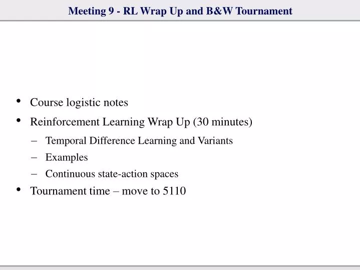
Meeting 9 - RL Wrap Up and B&W Tournament. Course logistic notes Reinforcement Learning Wrap Up (30 minutes) Temporal Difference Learning and Variants Examples Continuous state-action spaces Tournament time – move to 5110. Course Logistics. Course website: www.cim.mcgill.ca/~yon/ai

E N D
Meeting 9 - RL Wrap Up and B&W Tournament • Course logistic notes • Reinforcement Learning Wrap Up (30 minutes) • Temporal Difference Learning and Variants • Examples • Continuous state-action spaces • Tournament time – move to 5110
Course Logistics • Course website: www.cim.mcgill.ca/~yon/ai • WebCT Vista: • Course, project, assignment related discussion • Schedule office hours and assignment demo with TA (or write dcasto4@cim.mcgill.ca ) • Trottier 5110 Lab (assignment 1): • Graduate / exchange students: If you don’t already have access, you will need to submit your ID / DAS numbers to admin@cim.mcgill.ca . Mention this class.
Reinforcement Learning Problem • At each discrete time t, the agent observes state st∈ S and chooses action at∈ A • Then it receives immediate reward rt+1and the state changes to st+1
Models for MDPs • rsa is the expected value of the immediate reward if the agent is in s and performs action a: • pass’ is the probability of going from s to s’ when doing action a: • These form the model of the environment, and may be unknown
Policy • Execute actions in environment, observe results, and learnpolicyπ: S ×A → [0, 1] • Deterministic policy, π: S → A withπ(s) = a
Returns • Sequence of rewards received after t: rt+1, rt+2, rt+3 ... • Return Rt is the net reward received in the long run: • Finite-length tasks: • Continuing tasks (0 ≤ γ ≤ 1 is the discount factor):
Value and Action-Value Functions • ValueVof a state: the expected return starting from that state, when following the policy: • Action-ValueQ of a state: Expected return when starting in that state, taking the action, and following π afterwards (action-value function):
Learning • The main problems of RL can be stated as: • What is the value function Vπ or Qπof a given policy π? • How should we change π to improve the value function (closer to optimal V*)?
Action Value from Value Function • Simple relation to compute action-value function Q from value V, provided we have a model (r, p) of the environment:
Convergence of Bellman Equations • Error controlled by gamma:
Monte-Carlo Value Estimation • Agent behaves according to π for a while, generating several trajectories • Vπ(s) computed by averaging observed returns after s on trajectories in which s was visited • Average may be computed as each new trajectory is seen, using a “leaky accumulator”: • This can be regarded as modifying V with each new trajectory by an amount α in the direction of the true value R • Typically choose αt = 1 / n(st) to guarantee convergence.
Optimal Value Functions • Value gives partial order on policies: π ≥ π’ iff Vπ(s) ≥ Vπ’(s) ∀s • Optimal state-value function is the value function shared by all optimal policies: • Likewise, optimal action-value function: • Expected value for taking action a in state s and following an optimal policy afterwards
Bellman Equation for Optimal Value Function V* • The value of a state under the optimal policy must be equal to the expected return for the best action in the state: • V* is the unique solution to this system of non-linear equations
Bellman Equation for Optimal Action-Value Function Q* • Q* is the unique solution to this system of nonlinear equations
Why Care About Optimal Value Functions? • Any policy that is greedy with respect to V* is an optimal policy: • If we know V* and the model of environment, a search just one step ahead will tell us what the optimal action is (and so determine the policy). This is as we discussed in heuristic search. • If we know Q*, a one step search is not even needed; just set:
Policy Improvement • Given Vπfor some deterministic policy π. How to find a better policy? • Best clue: sometimes it is better to do an action a ≠ π(s), i.e. when: • Qπ(s,a) > Vπ(s) • If we make such a change at all states, we get a policy which is greedy with respect to Qπ : • Then Vπ’(s) ≥ Vπ(s), ∀ s⇒policy is better!
Policy Improvement • If at some point Vπ’ = Vπ, then we have • This is the Bellman optimality equation!!!! • Thus, if the value does not change at some point in the process of greedy improvement, both π and π’ are optimal.
Policy Iteration (for policy improvement) • Start with an initial policy π0 • Repeat: • Compute Vπk using policy evaluation • Compute a new policy πk+1 that is greedy with respect to Vπi: • Until Vπk = Vπk+1
Generalized Policy Iteration (for policy improvement) • Any combination of policy evaluation and policy improvement steps, even if they are not complete:
Value Iteration • Main idea: turn the Bellman optimality equation into an update rule (same as done in policy evaluation): • Start with an arbitrary initial approximation V0 • Vk+1←maxarsa +γ ∑s’ pass’ Vk (s’) , ∀ s
Monte-Carlo vs. Dynamic Programming • Monte-Carlo: • Dynamic Programming:
Dynamic Programming vs. Monte Carlo Value Estimation • Can we combine the advantages of both methods?
Value Estimation and Greedy Policy Improvement: Exercise • The exercise will posted in elaborated form on Friday 27 January on the course website. • The exercise will be due on Tuesday 7 February at 16h00. • This will count as one quiz toward your grade.
Monte-Carlo vs. Dynamic Programming • Monte-Carlo: • Dynamic Programming:
Combining Monte-Carlo and Dynamic Programming • Idea: use sampling idea of Monte-Carlo, but instead of nudging V in the direction of the true observed return Rt use estimate for the return: • The value function update formula becomes: • Note: if V(st+1) were a perfect estimate, this would be a DP update • This Value Estimation method is called Temporal-Difference (TD) learning
Temporal-Difference (TD) Learning • Like DP, it bootstraps (computes the value of a state based on estimates of the successors • Like MC, it estimates expected values by sampling
TD Learning: Advantages • No model of the environment (rewards, probabilities) is needed • TD only needs experience with the environment. • On-line, incremental learning • Both TD and MC converge. TD converges faster • Learn before knowing final outcome • Less memory and peak computation required
TD for learning action values • TD for value function learning: • Easy ansatz provides a TD version of action-value learning – • Bellman equation for Q: • Dynamic programming update for Q: • TD update for Q(s,a):
On-Policy SARSA learning • Policy improvement: At each time-step, choose action greedy mostly greedy with respect to Q: • After getting reward, seeing st+1, and choosing at+1, update action values:
Continuous (or large) state spaces • Previously considered that values held in table • Impractical for continuous or large (multi-dimensional) state spaces • Examples: Chess (~10^43), Robot manipulator (continuous) • Basic approaches: • Quantize continuous state spaces • Quantization of continuous state variables, perhaps coarse • Example: Angle in cart-pole problem quantized to (-90, -30, 0, 30, 90)° • Tilings: Impose overlapping - grid • More general approach: function approximation • Simple case: represent V(s) as a set of weights wi and basis functions fi(s) • V(s) = w1 f1(s) + w2 f2(s) + ... + wn fn(s) • Other methods of function approximation (eg. neural network) in coming weeks • Added benefit: V(s) able to predict value of states not yet visited
Robot that learns to stand • No static solution here to stand-up problem: robot must use momentum to stand up • RL used: • Two-layer heirarchy • TD learning for action values Q(s,a) applied to plan problem sub-goal sequence that may lead to success • Continuous version of TD learning applied to learn to achieve sub-goals • Robot trained several hundred iterations in simulation + 100 or so trials on the physical robot • Details: • J. Morimoto, K. Doya, “Acquisition of stand-up behavior by a real robot using heirarchical reinforcement learning”. J. Robotics Auto. Sys. 36 (2001)
Robot that learns to stand • After several hundred attempts in simulation
Robot that learns to stand • After ~100 hundred additional trials on robot
Wrap up • Next time: Wrap up of RL • Temporal Difference Learning • TD-Learning for Action-Values • Examples
Wrap up • Required readings • Russell and Norvig • Chapter 17, 21: Reinforcement learning • Optional but highly recommended (via course outline): • Sutton and Barto, Reinforcement Learning, pt 1(MIT Press, 1998) • (Link to HTML version from course readings) • Kaelbling et al., “Reinforcement Learning: A Survey” (1996) • Tesauro, “Temporal Difference Learning and TD-Gammon” (1995) • Acknowledgements: • Rich Sutton, Doina Precup, RL materials used here • Jeremy Cooperstock, AI Course Materials (2003)