Download
1 / 7
70 likes | 161 Vues
Solution under inputs. Solution under initial conditions. 9. Solution of a Set of Linear Differantial Equations. x : Column matrix of state variables (nx1). A: Square matrix (nxn), system matrix. u: Input vector (mx1). B: Input matrix (nxm). x 0 = {x} t=0. I: nxn unit matrix. L 2. L 1.

E N D
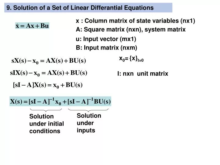
Solution under inputs Solution under initial conditions 9. Solution of a Set of Linear Differantial Equations x : Column matrix of state variables (nx1) A: Square matrix (nxn), system matrix u: Input vector (mx1) B: Input matrix (nxm) x0={x}t=0 I: nxn unit matrix
L2 L1 y2 y1 G yA yB c k c k m,I Example 9.1 (System in Problem 4 of Homework 01C) General Coordinates: y1, y2 Inputs: yA, yB m=1050 kg, I=670 kg-m2 k=35300 N/m, c=2000 Ns/m L1=1.7 m, L2=1.4 m M
clc;clear;syms s; a=[0,0,1,0 0,0,0,1 -185.9,91.8,-10.5,5.2 91.8,-136.5,5.2,-7.8]; eig(a) pause i1=eye(4);a1=inv(s*i1-a);pretty(a1) For multiplying polinoms, use conv ( ) commands in MATLAB
L2 L1 y2 y1 G yA yB c k c k m,I 0.05m (L=L1+L2=3.1 m)
L2 L1 y2 y1 G yA yB c k c k m,I 0.05m (ξ =0.45) (ξ =0.23) Δt=0.02, t∞=3.31 In input t1=0.186