Download

1 / 32
360 likes | 713 Vues
Poles and Zeros and Transfer Functions. Transfer Function:. A transfer function is defined as the ratio of the Laplace transform of the output to the input with all initial conditions equal to zero. Transfer functions are defined only for linear time invariant systems. Considerations :.

E N D
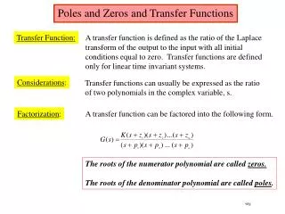
Poles and Zeros and Transfer Functions Transfer Function: A transfer function is defined as the ratio of the Laplace transform of the output to the input with all initial conditions equal to zero. Transfer functions are defined only for linear time invariant systems. Considerations: Transfer functions can usually be expressed as the ratio of two polynomials in the complex variable, s. Factorization: A transfer function can be factored into the following form. The roots of the numerator polynomial are called zeros. The roots of the denominator polynomial are called poles. wlg
Poles, Zeros and the S-Plane An Example: You are given the following transfer function. Show the poles and zeros in the s-plane. j axis S - plane origin x o x o x axis -14 -10 -8 -4 0 wlg
Poles, Zeros and Bode Plots Characterization: Considering the transfer function of the previous slide. We note that we have 4 different types of terms in the previous general form: These are: Given the tranfer function: Expressing in dB: wlg
Poles, Zeros and Bode Plots Mechanics: We have 4 distinct terms to consider: 20logKB 20log|(jw/z +1)| -20log|jw| -20log|(jw/p + 1)| wlg
1 1 1 1 1 1 This is a sheet of 5 cycle, semi-log paper. This is the type of paper usually used for preparing Bode plots. dB Mag Phase (deg) wlg (rad/sec)
Poles, Zeros and Bode Plots Mechanics: • The gain term, 20logKB, is just so many • dB and this is a straight line on Bode paper, • independent of omega (radian frequency). • The term, - 20log|jw| = - 20logw, when plotted • on semi-log paper is a straight line sloping at • 20dB/decade. It has a magnitude of 0 at w = 1. -20db/dec 20 0 -20 =1 wlg
Poles, Zeros and Bode Plots Mechanics: • The term, - 20log|(jw/p + 1), is drawn with the • following approximation: If w < p we use the • approximation that –20log|(jw/p + 1 )| = 0 dB, • a flat line on the Bode. If w > p we use the • approximation of –20log(w/p), which slopes at • -20dB/dec starting at w = p. Illustrated below. • It is easy to show that the plot has an error of • 3dB at w = p and – 1 dB at w = p/2 and w = 2p. • One can easily make these corrections if it is • appropriate. 20 0 -20db/dec -20 -40 = p wlg
Poles, Zeros and Bode Plots Mechanics: When we have a term of 20log|(jw/z + 1)| we approximate it be a straight line of slop 0 dB/dec when w < z. We approximate it as 20log(w/z) when w > z, which is a straight line on Bode paper with a slope of + 20dB/dec. Illustrated below. 20 +20db/dec 0 -20 -40 = z wlg
Example 1: Given: First: Always, always, always get the poles and zeros in a form such that the constants are associated with the jw terms. In the above example we do this by factoring out the 10 in the numerator and the 500 in the denominator. When you have neither poles nor zeros at 0, start the Bode at 20log10K = 20log10100 = 40 dB in this case. Second: wlg
Example 1: (continued) Third:Observe the order in which the poles and zeros occur. This is the secret of being able to quickly sketch the Bode. In this example we first have a pole occurring at 1 which causes the Bode to break at 1 and slope – 20 dB/dec. Next, we see a zero occurs at 10 and this causes a slope of +20 dB/dec which cancels out the – 20 dB/dec, resulting in a flat line ( 0 db/dec). Finally, we have a pole that occurs at w = 500 which causes the Bode to slope down at – 20 dB/dec. We are now ready to draw the Bode. Before we draw the Bode we should observe the range over which the transfer function has active poles and zeros. This determines the scale we pick for the w (rad/sec) at the bottom of the Bode. The dB scale depends on the magnitude of the plot and experience is the best teacher here. wlg
Bode Plot Magnitude for 100(1 + jw/10)/(1 + jw/1)(1 + jw/500) 1 1 1 1 1 1 1 1 1 1 1 1 60 4 0 20 dB Mag Phase (deg) dB Mag Phase (deg) 0 -20 -60 -60 (rad/sec) 0.1 1 10 100 1000 10000 (rad/sec) wlg
Using Matlab For Frequency Response Instruction: We can use Matlab to run the frequency response for the previous example. We place the transfer function in the form: The Matlab Program num = [5000 50000]; den = [1 501 500]; Bode (num,den) In the following slide, the resulting magnitude and phase plots (exact) are shown in light color (blue). The approximate plot for the magnitude (Bode) is shown in heavy lines (red). We see the 3 dB errors at the corner frequencies. wlg
1 10 100 500 Bode for: wlg
Phase for Bode Plots Comment: Generally, the phase for a Bode plot is not as easy to draw or approximate as the magnitude. In this course we will use an analytical method for determining the phase if we want to make a sketch of the phase. Illustration: Consider the transfer function of the previous example. We express the angle as follows: We are essentially taking the angle of each pole and zero. Each of these are expressed as the tan-1(j part/real part) Usually, about 10 to 15 calculations are sufficient to determine a good idea of what is happening to the phase. wlg
Bode Plots Example 2: Given the transfer function. Plot the Bode magnitude. Consider first only the two terms of Which, when expressed in dB, are; 20log100 – 20 logw. This is plotted below. The is 40 a tentative line we use until we encounter the first pole(s) or zero(s) not at the origin. -20db/dec 20 dB 0 -20 wlg (rad/sec) 1
Bode Plots Example 2: (continued) The completed plot is shown below. 1 1 1 1 1 1 60 60 -20db/dec 40 40 20 20 Phase (deg) Phase (deg) -40 db/dec dB Mag dB Mag 0 0 -20 -20 -40 -40 -60 -60 0.1 0.1 1 10 100 1000 1 10 100 1000 wlg (rad/sec) (rad/sec)
Bode Plots Example 3: Given: 20log80 = 38 dB 1 1 1 1 1 1 -60 dB/dec 60 40 dB Mag -40 dB/dec 20 0 -20 . wlg 1 10 0.1 100 (rad/sec)
Bode Plots Example 4: Given: 1 1 1 1 1 1 60 40 + 20 dB/dec -40 dB/dec 20 Phase (deg) dB Mag 0 Sort of a low pass filter -20 -40 -60 2 0.1 1 10 100 1000 wlg (rad/sec)
Bode Plots Given: Example 5 1 1 1 1 1 1 60 40 20 Phase (deg) dB Mag 0 -40 dB/dec Sort of a low pass filter -20 + 40 dB/dec -40 -60 0.1 1 10 100 1000 wlg (rad/sec)
Bode Plots Given: problem 11.15 text Example 6 . -40dB/dec . 40 -20db/dec . 20 -40dB/dec dB mag 0 . -20 -20dB/dec . -40 0.11 10 100 1000 wlg 0.01
Bode Plots Design Problem: Design a G(s) that has the following Bode plot. Example 7 40 30 dB -40dB/dec 20 +40 dB/dec 0 dB mag ? ? 30 900 0.1 1 10 100 1000 wlg rad/sec
Bode Plots Procedure: The two break frequencies need to be found. Recall: #dec = log10[w2/w1] Then we have: (#dec)( 40dB/dec) = 30 dB log10[w1/30] = 0.75 w1 = 5.33 rad/sec Also: (-40dB/dec) = - 30dB log10[w2/900] This gives w2 = 5060 rad/sec wlg
Bode Plots Procedure: Clearing: Use Matlab and conv: N1 = [1 10.6 28.1] N2 = [1 10120 2.56e+7] N = conv(N1,N2) 1 1.86e+3 2.58e+7 2.73e+8 7.222e+8 s4 s3 s2 s1 s0 wlg
Bode Plots Procedure: The final G(s) is given by; We now want to test the filter. We will check it at = 5.3 rad/sec And = 164. At = 5.3 the filter has a gain of 6 dB or about 2. At = 164 the filter has a gain of 30 dB or about 31.6. We will check this out using MATLAB and particularly, Simulink. Testing: wlg
Filter Output at = 5.3 rad/sec Produced from Matlab Simulink wlg
Filter Output at = 70 rad/sec Produced from Matlab Simulink wlg
Reverse Bode Plot Required: From the partial Bode diagram, determine the transfer function (Assume a minimum phase system) Example 8 Not to scale 68 20 db/dec -20 db/dec 30 20 db/dec dB 1 110 850 wlg
Reverse Bode Plot Required: From the partial Bode diagram, determine the transfer function (Assume a minimum phase system) Example 9 100 dB -40 dB/dec Not to scale 50 dB -20 dB/dec -20 dB/dec 10 dB -40 dB/dec 0.5 40 300 wlg w (rad/sec)
1 1 1 1 1 1 dB Mag Phase (deg) (rad/sec)