Download
1 / 31
310 likes | 494 Vues
Surface Simplification Using Quadric Error Metrics. Michael Garland Paul S. Heckbert. Why Simplification?. Full complexity of models is not always required Reduce the computational cost Get fast processing speed. Objective.

E N D
Surface Simplification Using Quadric Error Metrics Michael Garland Paul S. Heckbert
Why Simplification? • Full complexity of models is not always required • Reduce the computational cost • Get fast processing speed
Objective • Find a surface simplification algorithm that can be used in rendering systems for multiresolution model • Efficient • Good quality • Generality • Join unconnected regions of the model together ---- aggregation
Categories of surface simplification algorithms • Vertex Decimation • Vertex Clustering • Iterative Edge Contraction
Vertex Decimation • Basic idea • Iteratively selects a vertex for removal, removes all adjacent faces, and retriangulates the resulting hole. • Pros: provide reasonable efficiency and quality • Cons: only limited to manifold surfaces
Vertex Clustering • Basic idea • A bounding box is placed around the original model and divided into grids • Vertices within each cell are clustered together into a single vertex and model faces are updated accordingly • Pros: • Fast • Can make drastic topological alterations • Cons • Output quality is very low
Iterative Edge Contraction • Cons: do not support aggregation
Assumptions • Model only consists of triangles • The topology of the model need not to be maintained • In a good approximation, points do not move far from their original positions
Algorithm overview • Iteratively contract vertex pairs ( a generalization of edge contraction) • As the algorithm proceeds, a geometric error approximation is maintained at each vertex of the model which is represented using quadric matrices • The algorithm proceeds until the simplification goals are satisfied.
Advantages of pair contraction • Achieve aggregation, which can join previously unconnected regions of the model together • Algorithm is less sensitive to the mesh connectivity of the original model
Edge contraction vs. pair contraction Regular grid of 100 closely spaced cubes Approximation using edge contraction Approximation using pair contraction
Pair Selection • Select the set of valid pairs at initialization time • A pair (V1, V2) is a valid pair for contraction if either: • (V1, V2) is an edge, or • ||V1 – V2|| < t, where t is a threshold parameter
Pair contraction • Initially, each vertex is associated with the set of pairs of which it is a member • After performing contraction (V1, V2) → V1 • V1 acquires all the edges that were linked to V2 • Merge the set of pairs from V2 into its own set and remove duplicate pairs
Error approximation • Associate a symmetric 44 matrix Q with each vertex • The error at vertex v is defined as the quadratic form: ∆(v) = vTQv. • For a given contraction (v1, v2) → v’, a new matrix Q’ needs to be derived to approximate the error at v’. • Q’ = Q1 + Q2
Find the position for v’ • Simply select either v1, v2, or (v1+v2)/2 which produces the lowest value of error at v’ (∆(v’) = v’TQ’v’). • Find a position for v’ which minimizes ∆(v’)
Compute the initial Q matrices • Associate a set of planes with each vertex • Define the error of the vertex as the sum of squared distances to the planes Here p=[a b c d]T represents the plane defined by equation ax+by+cz+d=0, and a2+b2+c2=1
Quadratic form Kp is defined as “fundamental error quadric”.
Algorithm summary • Compute the Q matrices for all the initial vertices • Select all valid pairs and compute the optimal contraction target v’ for each valid pair (v1, v2). • The cost of contracting the pair is computed as: v’T(Q1+Q2)V’ • Place all the pairs in a heap keyed on cost with the minimum cost pair at the top • Iteratively remove the pair (v1, v2) of the least cost from the heap, contract this pair and update the costs of all valid pairs involving v1, v2.
Approximation evaluation • The approximation error Ei of the simplified model Mi is defined as: Mn ---- the initial model. Xn ---- sets of points sampled on model Mn Xi ---- sets of points sampled on model Mi
Result(1) ---- an example sequence of approximations 5,804 faces 994 faces 532 faces 248 faces 64 faces An example sequence of approximations generated by the algorithm. The entire sequence was constructed in about one second.
Result(2) – sample running times Time needed to make a 10 face approximation of the given model.
Result(3) – effect of optimal vertex placement Choosing an optimal position can significantly reduce approximation error.
Result(4) ---- bunny model 69,451 triangles 1,000 triangles 100 triangles 1.4% of original size 0.14% of original size
Result(5) ---- Terrain model 199,114 faces 999 faces (46 secs)
Result(6) ---- comparison between different methods Original model Edge Contractions (250 faces) (4,204 faces) Uniform Vertex Clustering Pair Contractions (250 faces) (262 faces)
Result(7) ---- level surfaces of error quadrics 1000 face approximation 250 face approximation
Conclusion • This paper presents a surface simplification algorithm using iterative pair contractions and quadric error metrics. • The algorithm can provide high efficiency, high quality and high generality.
Future works • Use a more sophisticated adaptive scheme to select valid pairs • Take the color of surface into account