Download
1 / 119
1.28k likes | 2.13k Vues
INTERNAL INCOMPRESSIBLE VISCOUS FLOW. Nazaruddin Sinaga Laboratorium Efisiensi dan Konservasi Energi Universitas Diponegoro. Outline. Flow Measurements. Osborne Reynolds Experiment. Laminar and Turbulent Flow. Entrance Length. Developing Flow. 2. 1. 5. Types of Flow.

E N D
INTERNAL INCOMPRESSIBLE VISCOUS FLOW Nazaruddin Sinaga Laboratorium Efisiensi dan Konservasi Energi Universitas Diponegoro
Outline • Flow Measurements
2 1 5
Types of Flow • The physical nature of fluid flow can be categorized into three types, i.e. laminar, transition and turbulent flow. Reynolds Number (Re) can be used to characterize these flow. (6.3) where = density = dynamic viscosity = kinematic viscosity ( = /) V = mean velocity D = pipe diameter In general, flow in commercial pipes have been found to conform to the following condition: Laminar Flow: Re <2000 Transitional Flow : 2000 < Re <4000 Turbulent Flow : Re >4000
Laminar Flow • Viscous shears dominate in this type of flow and the fluid appears to be moving in discreet layers. The shear stress is governed by Newton’s law of viscosity • In general the shear stress is almost impossible to measure. But for laminar flow it is possible to calculate the theoretical value for a given velocity, fluid and the appropriate geometrical shape.
Pressure Loss During A Laminar Flow In A Pipe - In reality, because fluids are viscous, energy is lost by flowing fluids due to friction which must be taken into account. • - The effect of friction shows itself as a pressure (or head) loss. In a pipe with a real fluid flowing, the shear stress at the wall retard the flow. • - The shear stress will vary with velocity of flow and hence with Re. Many experiments have been done with various fluids measuring the pressure loss at various Reynolds numbers. • - Figure below shows a typical velocity distribution in a pipe flow. It can be seen the velocity increases from zero at the wall to a maximum in the mainstream of the flow. A typical velocity distribution in a pipe flow
In laminar flow the paths of individual particles of fluid do not cross, so the flow may be considered as a series of concentric cylinders sliding over each other. • Lets consider a cylinder of fluid with a length L, radius r, flowing steadily in the center of pipe. Cylindrical of fluid flowing steadily in a pipe
The fluid is in equilibrium, shearing forces equal the pressure forces. Shearing force = Pressure force (6.5) Taking the direction of measurement r (measured from the center of pipe), rather than the use of y (measured from the pipe wall), the above equation can be written as; (6.6) Equatting (6.5) with (6.6) will give:
In an integral form this gives an expression for velocity, with the values of r = 0 (at the pipe center) to r = R (at the pipe wall) (6.7) where P = change in pressure L = length of pipe R = pipe radius r = distance measured from the center of pipe The maximum velocity is at the center of the pipe, i.e. when r = 0. It can be shown that the mean velocity is half the maximum velocity, i.e. V=umax/2
The discharge may be found using the Hagen-Poiseuille equation, which is given by the following; (6.8) The Hagen-Poiseuille expresses the discharge Q in terms of the pressure gradient , diameter of pipe, and viscosity of the fluid. Pressure drop throughout the length of pipe can then be calculated by (6.9) Shear stress and velocity distribution in pipe for laminar flow
Fully Developed Laminar Flowin a Pipe • Velocity Distribution • Shear Stress Distribution
Fully Developed Laminar Flowin a Pipe • Volume Flow Rate • Flow Rate as a Function of Pressure Drop
Fully Developed Laminar Flowin a Pipe • Average Velocity • Maximum Velocity
Turbulent Flow • This is the most commonly occurring flow in engineering practice in which fluid particles move erratically causing instantaneous fluctuations in the velocity components. • These fluctuations cause additional shear stresses. In this type of flow both viscous and turbulent shear stresses exists. • Thus, the shear stress in turbulent flow is a combination of laminar and turbulent shear stresses, and can be written as: where = dynamic viscosity = eddy viscosity which is not a fluid property but depends upon turbulence condition of flow.
The velocity at any point in the cross-section will be proportional to the one-seventh power of the distance from the wall, which can be expressed as: (6.10) where Uy is the velocity at a distance y from the wall, UCL is the velocity at the centerline of pipe, and R is the radius of pipe. This equation is known as the Prandtl one-seventh law. Figure below shows the velocity profile for turbulent flow in a pipe. The shape of the profile is said to be logarithmic. Velocity profile for turbulent flow
For smooth pipe: (6.11a) • For rough pipe: (6.11b) In the above equations, U represents the velocity at a distance y from the pipe wall, U* is the shear velocity = y is the distance form the pipe wall, k is the surface roughness and is the kinematic viscosity of the fluid.
Head Losses The momentum balance in the flow direction is thus given by