Download
1 / 26
260 likes | 393 Vues
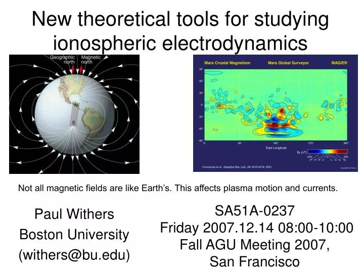
New theoretical tools for studying ionospheric electrodynamics. Paul Withers Boston University (withers@bu.edu). Not all magnetic fields are like Earth’s. This affects plasma motion and currents. SA51A-0237 Friday 2007.12.14 08:00-10:00 Fall AGU Meeting 2007, San Francisco. Motivation.

E N D
New theoretical tools for studying ionospheric electrodynamics Paul Withers Boston University (withers@bu.edu) Not all magnetic fields are like Earth’s. This affects plasma motion and currents. SA51A-0237 Friday 2007.12.14 08:00-10:00 Fall AGU Meeting 2007, San Francisco
Motivation • I want a model that can predict ion densities Njand velocities vj • Nj is given by the continuity equation • Rate of change of Nj= Production - Loss • vj is given by the steady-state momentum equation • Gravity Pressure gradient Lorentz force Ion-neutral collisions • Model needs the electric field E. How can E be predicted?
How to Find the Electric Field E • Empirical model • Useless beyond Earth, not based on first-principles • Ambipolar diffusion • Assume that current density J = 0, which lets you solve for E. Works when magnetic field is either very weak or very strong by comparison to the effects of collisions. Does not work for general magnetic field strengths. • Use dynamo theory, Maxwell’s equations, and boundary conditions to solve for E. neglects gravity and pressure gradients, so this is useless when plasma motion is not purely horizontal. • These possible approaches work well for the special case of Earth, but are not completely general. In particular, none of them can describe the vertical motion of plasma in a dynamo region, where electrons, but not ions, are bound to fieldlines. This matters for Mars.
Why lack of generality has not been considered a problem for terrestrial ionospheric research • Vertical transport of plasma in the terrestrial ionosphere is only important where ions/electrons are frozen to fieldlines • Vertical transport important where transport timescales are shorter than photochemical timescales, F region and above • Freezing in of ions/electrons to magnetic fieldlines is controlled by ratio of gyrofrequency to collision frequency • What if ions/electrons became frozen to fieldlines in the middle of the F region, instead of at much lower altitudes? • Could occur on Earth if B was weaker • Does occur on other planets (Mars) • Neither weak field nor strong field limits of ambipolar diffusion are useful in this case of intermediate field strength • neglects gravity and pressure gradients, which drive vertical transport, so it is not useful
Goal of Research Project • Obtain a more general way of modelling ion velocities • Valid for arbitrary magnetic field strength • Valid for horizontal, vertical, or mixed motion • Valid for flow of current and bulk motion of plasma • Start by getting a general relationship between J and E’ • Then apply model to Mars-like situation
Abstract Two different theoretical approaches are commonly used to study ionospheric plasma motion. Dynamo theory and the conductivity equation is used to study currents caused by plasma motion. Ambipolar diffusion models are used to study changes in plasma density caused by vertical plasma motion. The conductivity equation, which states that the current density vector equals the product of the conductivity tensor and the electric field vector, is derived from the conservation of momentum equations after the effects of gravity and pressure gradients are neglected. These terms are crucial for ambipolar diffusion. The two different theoretical approaches are inconsistent. On Earth, the dynamo region (75 km to 130 km, altitude controlled by magnetic field strength and collision frequencies) occurs below regions (F region) where ambipolar diffusion affects plasma number densities, so the theoretical inconsistencies are rarely noticed. However, the inconsistencies are present in most thermosphere-ionosphere-electrodynamics models and will affect the results of such models, particularly in the F region. We present an extension of the conductivity equation that can self-consistently describe ionospheric currents and plasma diffusion.
The Basic Equations Momentum equation (above) and definition of current density J (left) Algebraic Simplifications Change of variables vj (left) and E (centre) and quasi-neutrality condition (right) Revised Basic Equations Revised momentum equation (above) and definition of current density J (left)
Mathematical problems with B If there are p species of ions, then there are p+2 equations linking the p+3 unknowns J, E’, and wj Thus there must be a linear relationship between J and E’ Problem: The vector cross product involving B cannot be inverted, so how can an equation linking J and E’ be found? Solution: Define matrix by for any vector
Relationship between J and E’ This equation for wj and can be used to find an equation linking J and E’ (Compare to ) Ratio of gyrofrequency to collision frequency Gravity and Pressure gradient Direction depends on Kj
and the Conductivity Tensor Assume that B is parallel to z-axis to compare and the usual representation of As shown below, and are equivalent, so is a frame-independent representation of the conductivity tensor reduces to when gravity and pressure gradient forces are neglected.
Using in a 1-D model – Step 1 • and can be combined to give where R and are known • Ex, Ey are uniform • Jz is uniform • If either J or E is specified on model’s lower boundary, then can be used to find the other vector (E or J) on that boundary
Using in a 1-D model – Step 2 • Use Jz = Rz + Szx Ex + Szy Ey + Szz Ez to find Ez at all altitudes • Hence E, E’, J can be found at all altitudes • wj and vj can also be found from previous equations • Induced magnetic field can also be found from (subject to boundary condition)
Application to a Simplified Mars-Like Ionospheric Model – Step 1 • Neutral atmosphere is CO2 with scale height of 12 km and number density of 1.4E12 cm-3 at 100 km. • Gravity = 3.7 ms-2 • Flux of ionizing photons at 1 AU is 5E10 cm-2 s-1 and Mars at 1.5 AU from the Sun • Absorption/ionization cross-section of CO2 molecules is 1E-17 cm2 • Each photon absorbed leads to the creation of one O2+ ion • Dissociative recombination coefficient is 2E-7 cm3 s-1
Application to a Simplified Mars-Like Ionospheric Model – Step 2 • Dissociative recombination coefficient is 2E-7 cm3 s-1 • Ion-neutral and electron-neutral collision frequencies from Banks and Kockarts • Magnetic field strength is 50 nT • Electrons frozen to fieldlines at >140 km, ions frozen to fieldlines at >200 km • Wind speed is zero • Lower boundary condition is J=0 at 100 km • Simplified chemistry is realistic for main ionospheric peak and below on Mars, but neglects O+ at higher altitudes • Simplified magnetic fields are realistic
Simulation 1 • Produce ionosphere using only photochemical processes, then suddenly switch transport processes on • Let I, inclination of B to horizontal, be 45o • What are the predicted ion and electron velocities at that instant? • Do they match the weak-field ambipolar solution at low altitudes and the strong-field ambipolar solution at high altitudes?
vz using (solid line), vz using weak-field limit of ambipolar diffusion (dashed line), and vz using strong-field limit of ambipolar diffusion (dotted line). vz is negative below 150 km and positive above 150 km. vz transitions smoothly from the weak-field limit at low altitudes to the strong-field limit at high altitudes.
-Jx (dashed line), Jy (dotted line) and |J| (solid line). Jz = 0. Ke = 1 at 140 km, Ki = 1 at 200 km |J| is >10% of its maximum value between 150 km and 260 km Currents are significant within and above the 140 km – 200 km “dynamo region”
Let qj = angle between velocity vector and B. qe (dashed line) and qi (solid line) qj = 00 -> motion parallel to B, qj = 1800 -> motion anti-parallel to B qj = 450 -> upwards motion, qj = 1350 -> downwards motion At low altitudes, neither ions nor electrons are tied to fieldlines (qi, qe = 450 or 1350) At high altitudes, both ions and electrons are tied to fieldlines (qi, qe = 00 or 1800) At intermediate altitudes (dynamo region), electrons, but not ions, are tied to fieldlines
Simulations 2.1 to 2.6 • Allow transport processes to reach steady state • Six cases: I = 15o, 30o, 45o, 60o, 75o, and 90o • B = 50 nT in all six cases • Upper boundary condition for vz is 5 km s-1 at 300 km for all six cases
N(z) for simulations 2.1 to 2.6. Values of I are 150, 300, 450, 600, 750, and 900. Large values of N at 300 km correspond to large values of I Small values of N at 230 km correspond to large values of I Differences in ion density occur above top of dynamo region (200 km) Ion densities can vary by tens of percent depending on I
N(z) for simulations 2.1 to 2.6. Values of I are 150, 300, 450, 600, 750, and 900. Large values of N at 300 km correspond to large values of I Small values of N at 230 km correspond to large values of I NPC is ion density profile for situation where plasma transport is turned off This figure highlights the relative differences in N more clearly than the previous figure.
vz(z) for simulations 2.1 to 2.6. Values of I are 150, 300, 450, 600, 750, and 900. Large values of vz at 240 km correspond to large values of I The same upper boundary condition, vz = 5 km s-1, was used in all six simulations The vertical component of ion velocity is very dependent on I. vz at 240 km varies by an order of magnitude in these six simulations.
Questions for the Audience • How would you calculate 3D electric fields, ion velocities, and current density self-consistently if the magnetic field is neither weak nor strong? • The conductivity tensor, , is supposed to be frame-independent, but textbooks always state it in a frame-dependent representation. Have you seen a frame-independent representation of ?
Terrestrial Implications • Weak-field ambipolar diffusion, strong-field ambipolar diffusion, and are all special cases of • Sophisticated terrestrial models, such as TIE-GCM, MTIE-GCM, CTIP, and CMIT, use the incomplete relationship in studies of electrodynamics and plasma transport • The usual MHD equations are also derived from
Summary • Techniques used in terrestrial ionospheric modelling to determine the electric field and its influence on 3D plasma motions and currents are not fully general. • They are not suitable when electrons are frozen in to fieldlines, but ions are not. • More general techniques are derived and demonstrated here.
Conclusions • has been used to model 3D currents and ion velocities for a Mars-like ionosphere. • Ion velocities are consistent with the weak-field limit of ambipolar diffusion at low altitudes, where the magnetic field is weak, and consistent with the strong-field limit of ambipolar diffusion at high altitudes, where the magnetic field is strong. • Ion velocities, currents, and electric fields are self-consistent.