Download
1 / 74
750 likes | 971 Vues
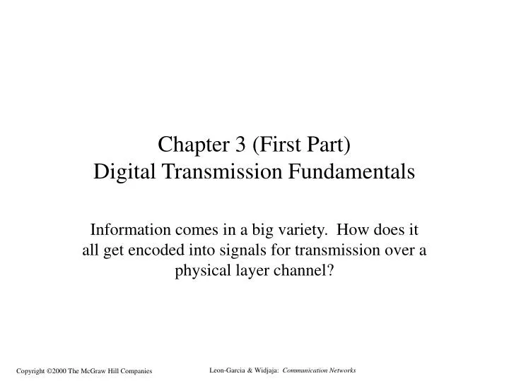
Chapter 3 (First Part) Digital Transmission Fundamentals. Information comes in a big variety. How does it all get encoded into signals for transmission over a physical layer channel?. Homework Discussion, Forecast of Domains and Optical System Performance 3.1 Digital Representation of Info

E N D
Chapter 3 (First Part)Digital Transmission Fundamentals Information comes in a big variety. How does it all get encoded into signals for transmission over a physical layer channel?
Homework Discussion, Forecast of Domains and Optical System Performance 3.1 Digital Representation of Info 3.2 Why Digital? Why not Analog? The basic sinewave and pulse train carrier signals Next Time 3.4 Fundamental Limits 3.5 Line Coding 3.6 Modems 3.3 Characterization of Communication Channels Outline For Today
Forecasting Internet growth from nw.com data Linear Scale. Tough to extrapolate since it is an exponential. Log Scale. Draw a line or use Excel LOGEST
Moore’s Law models progress in the IC chip business. Since 1960 number of bits on a chip has doubled every 18 months or so. How long will it continue? “Andreessen’s Law” models growth in Internet domain names. Since 1995 number of names has doubled every 18 months or so. Is this a coincidence? Both processes were foundations for rapid growth in jobs, products and services, and Wall St. speculation Can you estimate the doubling interval for optical communications from Fig. 1.9. Note the change in 1995-2000 with the invention of DWDM. Can this continue? Will there be another investment frenzy? Will there be another bust? Role of Exponential Growth in Making (I wrote this in 2000; how things have changed!)
Transmitter Receiver Communication channel The basic communications model Figure 3.5
Information comes in many forms, but we need to encode it into either an analog (continuously varying) or digital (two or M-level) signal for transmission Currently the digital option is preferred for new systems for several reasons. Computer processing is more flexible (software) vs. analog signal processing by electronic devices. We’ll see some more on the next few slides. Legacy systems like AM / FM radio, NSTC TV are very difficult to change to digital – Why? Why Digital Transmission?
(a) Analog transmission: all details must be reproduced accurately Analog vs. digital signal designs Received Sent • e.g. AM, FM, TV transmission (b) Digital transmission: only discrete levels need to be reproduced Received Sent • e.g digital telephone, CD Audio Figure 3.6
Often repeaters are used to send a signal over a long distance. Transmission segment Destination Source Repeater Repeater Figure 3.7
At each analog repeater, we amplify the received signal and noise. We amplify both: A[as(t) + n(t)] Suppose Aa =1. Recovered signal + residual noise Attenuated & distorted signal + noise Amp. Equalizer Repeater After n repeaters we have: s(t) + nAn(t); not good Figure 3.8
A digital repeater can perfectly reconstruct the transmitted signal Decision Circuit. & Signal Regenerator Amplifier Equalizer Timing Recovery Murphy’s brother’s-in-law Law: “Nothing is perfect.” What can go wrong here? Figure 3.9
SNR signal + noise signal noise High SNR t t t noise signal + noise signal Low SNR t t t Average Signal Power SNR = Average Noise Power SNR (dB) = 10 log10 SNR Figure 3.12
(a) 7D/2 5D/2 3D/2 D/2 Original and samples -D/2 -3D/2 -5D/2 Conversion of analog voice to digital. -7D/2 7D/2 (b) 5D/2 3D/2 Original and quantized values D/2 -D/2 -3D/2 -5D/2 -7D/2 Figure 3.2
W W W W H H H H Conversion of still pictures to digital Red Component Image Green Component Image Blue Component Image Color Image = + + Total bits before compression = 3xHxW pixels x B bits/pixel = 3HWB Figure 3.1
Conversion of video for digital transmission 176 (a) QCIF Videoconferencing 144 @ 30 frames/sec = 760,000 pixels/sec 720 (b)Broadcast TV @ 30 frames/sec = 10.4 x 106 pixels/sec 480 1920 (c) HDTV @ 30 frames/sec = 67 x 106 pixels/sec 1080 Figure 3.3
A digital channel d meters 0110101... communication channel 0110101... • How fast we can send digital information depends on: • Energy per bit • Distance • Noise • Bandwidth Figure 3.10
Role of Bandwidth (a) Lowpass and idealized lowpass channel A(f) A(f) 1 f f 0 W 0 W (b) Maximum pulse transmission rate is 2W pulses/second Channel t t Typical amplitude-response functions Figure 3.11
Aincos 2ft Aoutcos (2ft + (f)) Channel t t Aout Ain A(f) = Figure 3.13
h(t) Channel t t 0 td Figure 3.17
A(f)=1 1+42f2 1 f Figure 3.14 - Part 1
(f)=tan-1 2f 1/2 0 f -45o -90o Figure 3.14 - Part 2
Original sequence (a) 1 2 3 4 5 6 7 8 9 (b) Jitter due to variable delay 1 2 3 4 5 6 7 8 9 Playout delay (c) 1 2 3 4 5 6 Figure 3.4
1 0 0 0 0 0 0 1 . . . . . . t 1 ms Figure 3.15
s(t) = sin(2Wt)/ 2Wt t T T T T TT T T T TT T TT Figure 3.18
1 0 1 1 0 1 +A 2T 4T 5T T 3T 0 t -A r(t) Transmitter Filter Comm. Channel Receiver Filter Receiver Received signal Figure 3.19
(a) 3 separate pulses for sequence 110 t T T T T T T (b) Combined signal for sequence 110 t T T T T T T Figure 3.20
(1- )W W (1+ )W f 0 Figure 3.21
typical noise 4 signal levels 8 signal levels Figure 3.22
x 0 Figure 3.23
0 2 4 6 8 /2 Figure 3.24
0 1 0 1 1 1 1 0 0 Unipolar NRZ Polar NRZ NRZ-Inverted (Differential Encoding) Bipolar Encoding Manchester Encoding Differential Manchester Encoding Figure 3.25
f f2 f1 0 fc Figure 3.27
1 0 1 1 0 1 6T 6T 6T 2T 2T 2T 4T 4T 4T 5T 5T 5T 3T 3T 3T T T T 0 0 0 Information +1 (a) Amplitude Shift Keying t -1 +1 Frequency Shift Keying (b) t -1 +1 Phase Shift Keying (c) t -1 Figure 3.28
1 0 1 1 0 1 +A (c) Modulated Signal Yi(t) 6T 2T 4T 5T 3T T 0 -A 6T 2T 4T 5T 3T T 0 (a) Information +A (b) Baseband Signal Xi(t) t 6T 2T 4T 5T T 3T 0 -A t +2A (d) 2Yi(t) cos(2fct) t -2A Figure 3.29
(a) Modulate cos(2fct) by multiplying it by Akfor (k-1)T < t <kT: x Ak Yi(t) = Akcos(2fct) cos(2fct) (b) Demodulate (recover) Akby multiplying by 2cos(2fct) and lowpass filtering: Lowpass Filter with cutoff W Hz x Yi(t) = Akcos(2fct) Xi(t) 2cos(2fct) 2Akcos2(2fct) = Ak {1 + cos(2fct)} Figure 3.30
x Ak Yi(t) = Akcos(2fc t) cos(2fc t) + Y(t) x Bk Yq(t) = Bksin(2fc t) sin(2fc t) Modulatecos(2fct)and sin (2fct)bymultiplying them by Akand Bk respectively for (k-1)T < t <kT: Figure 3.31
Lowpass Filter with cutoff W/2 Hz x Y(t) Ak 2cos(2fc t) 2cos2(2fct)+2Bkcos(2fct)sin(2fct) = Ak {1 + cos(4fct)}+Bk{0 + sin(4fct)} Lowpass Filter with cutoff W/2 Hz x Bk 2sin(2fc t) 2Bk sin2(2fct)+2Akcos(2fct)sin(2fct) = Bk{1 - cos(4fct)}+Ak {0 + sin(4fct)} Figure 3.32
2-D signal Bk Ak 4 “levels”/ pulse 2 bits / pulse 2W bits per second Bk 2-D signal Ak 16 “levels”/ pulse 4 bits / pulse 4W bits per second Figure 3.33
Bk Bk Ak Ak 16 “levels”/ pulse 4 bits / pulse 4W bits per second 4 “levels”/ pulse 2 bits / pulse 2W bits per second Figure 3.34
Frequency (Hz) 106 108 1010 1012 1014 1016 1018 1020 1022 1024 102 104 power & telephone broadcast radio microwave radio gamma rays infrared light visible light ultraviolet light x rays 106 104 102 10 10-2 10-4 10-6 10-8 10-10 10-12 10-14 Wavelength (meters) Figure 3.35
d meters communication channel t = d/c t = 0 Figure 3.36
26 gauge 30 24 gauge 27 24 22 gauge 21 18 Attenuation (dB/mi) 19 gauge 15 12 9 6 3 f (kHz) 100 1000 1 10 Figure 3.37
Figure 3.38
Center conductor Dielectric material Braided outer conductor Outer cover Figure 3.39
35 0.7/2.9 mm 30 25 1.2/4.4 mm Attenuation (dB/km) 20 15 2.6/9.5 mm 10 5 0.01 0.1 10 100 f (MHz) 1.0 Figure 3.40
Head end Unidirectional amplifier Figure 3.41
Upstream fiber Fiber Fiber Head end Fiber node Fiber node Downstream fiber Coaxial distribution plant Bidirectional Split-Band Amplifier Figure 3.42
Downstream 54 MHz 500 MHz Downstream Upstream 42 MHz 5 MHz 54 MHz 500 MHz (a) Current allocation Proposed downstream (b) Proposed hybrid fiber-coaxial allocation 750 MHz 550 MHz Figure 3.43
light cladding jacket core c (a) Geometry of optical fiber (b) Reflection in optical fiber Figure 3.44