Download
1 / 40
400 likes | 403 Vues
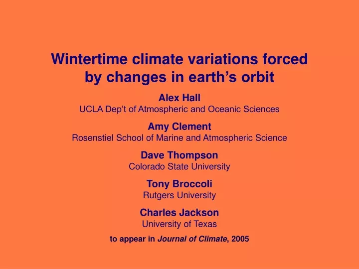
Wintertime climate variations forced by changes in earth’s orbit Alex Hall UCLA Dep’t of Atmospheric and Oceanic Sciences Amy Clement Rosenstiel School of Marine and Atmospheric Science Dave Thompson Colorado State University Tony Broccoli Rutgers University

E N D
Wintertime climate variations forced by changes in earth’s orbit Alex HallUCLA Dep’t of Atmospheric and Oceanic Sciences Amy ClementRosenstiel School of Marine and Atmospheric Science Dave ThompsonColorado State University Tony BroccoliRutgers University Charles JacksonUniversity of Texas to appear in Journal of Climate, 2005
obliquity varies on approximately a 40,000 year time scale. High obliquity means the high latitudes receive more insolation on an annual basis, while the tropics receive less.
The direction of the earth’s spin axis also precesses. This means that the earth’s spin axis traces out a circle. Like obliquity, precession occurs on very long time scales. It takes about 20,000 years for the spin axis to trace out a circle once.
The situation now. Aphelion occurs in early July and coincides with northern hemisphere summer. The situation about 10,000 years ago in the opposite phase of the earth’s precessional cycle. Aphelion occurs in early January and coincides with southern hemisphere summer.
Summary: how orbital variations affect sunshine Obliquity When obliquity is high, seasonality is enhanced. In mid and high latitudes, more sunshine comes in summer, and less comes in winter. Averaged over the whole year, the high latitudes receive more sunshine, and the low latitudes receive less. Precession When perihelion occurs at summer solstice, the contrast between summer and winter is enhanced. When perihelion occurs at winter solstice, seasonality is weakened. Precession has little effect on annual mean sunshine. Eccentricity Changes in the eccentricity of the earth’s orbit have very little effect on the annual mean sunshine anywhere. However, they do have a large impact on the amplitude of the precessional cycle. If the earth’s orbit is very eccentric, the timing of perihelion in the calendar year becomes more critical.
background Much internal climate variability stems from well-known modes of variability, such as ENSO (tropics) and the annular modes (extratropics) (e.g. Hurrell 1995, Hurrell et al. 2003; Kidson 1988; Karoly 1990; Hartmann and Lo 1998; Thompson and Wallace 2000). Like ENSO, the northern annular mode (NAM) is linked with significant variability in temperature and other climate variables because of its association with atmospheric circulation anomalies (e.g. Hurrell et al. 2003). ENSO’s dynamical response to orbital forcing has been proposed as an important component of paleoclimate variability (Clement et al. 1999). However, extratropical paleoclimate has not been viewed in terms of modes of variability. Attention has focused instead on the direct thermodynamic response to orbital forcing. (Hays et al. 1976; Imbrie et al. 1984) In this study, we demonstrate that NAM dynamics are crucial to the NH extratropical wintertime response of a climate model to orbital forcing.
experimental design We use an atmospheric general circulation model on a global domain coupled to a mixed layer ocean model (isothermal 50 m depth slab). The model has a resolution of approximately 4.5° latitude by 7.5° longitude (r15). There are nine vertical levels, with the top level coinciding roughly with a pressure of 25 hPa. Seasonal variations in deep ocean heat transport are included as a prescribed flux at the bottom of the ocean mixed layer. These heat fluxes are chosen to maintain present-day SSTs when the present-day orbital configuration is imposed. Sea ice dynamics and thermodynamics are included. Ice sheets are prescribed to the present-day configuration. We impose in continuous fashion insolation variations associated with changes in earth’s orbit of the past 165,000 yrs. (Berger, 1992) The orbital variations are accelerated by a factor of 30, so that the actual integration lasts only 5,500 yrs.
pressure anom. (hPa) 0 20 40 60 80 100 120 140 160 effective kyrs before present An example of a time series produced by the experiment. This shows wintertime (DJF) sea level pressure in the central North Atlantic (42N, 38W).
LEAST SQUARES FITTING PROCEDURE obliquity component residual component precessional component raw anomaly time series of any variable
LEAST SQUARES FITTING PROCEDURE obliquity component This is the portion of the model response that can be linearly related to obliquity. The fitting procedure determines Ao, the amplitude of the obliquity response. We do not allow climate variables to have a phase relationship with obliquity.
LEAST SQUARES FITTING PROCEDURE This is the portion of the model response that can be linearly related to precession. Because the precessional cycle has a continuously varying phase relationship with the annual cycle, we have to allow climate variables to have a phase as well as an amplitude relationship with precessional forcing. Example: SST The fitting procedure determines Ap, the amplitude of the precession response, as well as p, the phase of the response. precessional component
LEAST SQUARES FITTING PROCEDURE The residual component contains all the variability that cannot be linearly related to precession or obliquity. In principle, it is composed of: The nonlinear response to precession and obliquity Direct effects of the 100 kyr eccentricity cycle Internal climate variability residual component In practice, this component is overwhelmingly dominated by internal climate variability.
pressure anom. (hPa) 0 20 40 60 80 100 120 140 160 effective kyrs before present Now we show an example of an application of the least squares fitting procedure. We return to the time series of DJF sea level pressure in the central North Atlantic (42N, 38W).
pressure anom. (hPa) 0 20 40 60 80 100 120 140 160 effective kyrs before present total orbital component
pressure anom. (hPa) 0 20 40 60 80 100 120 140 160 effective kyrs before present
pressure anom. (hPa) effective kyrs before present
pressure anom. (hPa) “ORBITAL” “INTERNAL” effective kyrs before present
EOF PATTERN EOF TIME SERIES insolation--40N normalized anomaly 0 20 40 60 80 100 120 140 160 effective kyrs before present EOF analysis of summertime orbital and internal SLP variability.
EOF PATTERN EOF TIME SERIES normalized anomaly effective kyrs before present EOF analysis of wintertime orbital and internal SLP variability.
NH winter (DJF) The projection of zonal-mean zonal winds onto the primary mode of orbital SLP variability closely resembles the projection of zonal-mean zonal winds onto the primary mode of internal SLP variability. High NAM index is associated with an intensification of the jet stream poleward of about 45N, and a weakening equatorward of 45N. The anomalies in the zonal wind organize eddy activity such that the anomalies in the zonal flow are reinforced. (Lorenz and Hartmann 2003; Robinson 2000)
some background Robinson (2000) and Kushnir et al. (2002) argue that changes in the meridional surface temperature gradient in mid-latitudes induce changes in the NAM via the relationship between lower tropospheric baroclinicity and convergence of the eddy momentum flux in the upper troposphere. Along a latitude of enhanced meridional surface temperature gradient, there is increased generation of baroclinic eddies in the lower troposphere and thus increased momentum flux convergence in the upper troposphere as the eddies radiate away from their source latitude. The combined effects of anomalous heat and momentum fluxes by the eddies give rise to equivalent barotropic westerly anomalies. We invoke this mechanism to argue that orbitally-induced variations in the temperature gradient across the main axis of the westerly NAM anomalies near 55N are very likely the reason why the response to orbital forcing during NH winter is dominated by a NAM-like pattern.
Hovmuller diagram of the obliquity component of wintertime zonal-mean SST. The wintertime SSTs follow the annual-mean insolation anomaly due to obliquity, with warm temperatures at high latitudes and cool temperatures at low latitudes when obliquity is high.
Hovmuller diagram of the obliquity component of wintertime zonal-mean SST. The wintertime SSTs follow the annual-mean insolation anomaly due to obliquity, with warm temperatures at high latitudes and cool temperatures at low latitudes when obliquity is high. Time series of the obliquity component of zonal-mean wintertime SST gradient (difference in zonal-mean DJF SST between 38°N and 74°N), and the obliquity component of the time series of the primary mode of DJF SLP variability.
Hovmuller diagram of the precession component of wintertime zonal-mean SST. The largest anomalies are seen in low latitudes, where mean sunshine is the strongest. Here, SST reaches its maximum when perihelion occurs in October.
Hovmuller diagram of the precession component of wintertime zonal-mean SST. The largest anomalies are seen in low latitudes, where mean sunshine is the strongest. Here, SST reaches its maximum when perihelion occurs in October. Time series of the precession component of zonal-mean wintertime SST gradient, the precession component of the time series of the primary mode of DJF SLP variability, and October-mean solar forcing due to precession.
Projection of surface air temperature (C) onto the model’s internally-generated NAM Positive NAM is associated with warm anomalies over the North American continent and northwestern Eurasia, and cold anomalies over far eastern Siberia and the Labrador Sea. This is very similar to the SAT anomalies associated with the real atmosphere’s NAM. These have been traced to anomalies in the atmospheric circulation. (Hurrell 1995, Thompson and Wallace 2000)
Projection of surface air temperature (C) onto the model’s orbitally-generated NAM Though there is some similarity to the SAT impact of the internally-generated NAM, this pattern is almost certainly contaminated by the direct thermodynamic response to orbital forcing correlated with the orbital NAM time series. We hypothesize that this response has a zonally-symmetric structure, since the forcing is zonally-symmetric.
Projection of zonally-asymmetric anomalies in surface air temperature (C) onto the model’s orbitally-generated NAM The overwhelming similarity between this pattern and the internal case suggests our hypothesis is correct, and that the zonally-asymmetric SAT response to orbital forcing is the result of orbital NAM forcing.
EOF analysis of wintertime orbital SLP variability. EOF PATTERN EOF TIME SERIES normalized anomaly 0 20 40 60 80 100 120 140 160 effective kyrs before present The simulation is most directly applicable to the real climate for periods when the configuration of ice sheets was similar to the present. This is true during the Holocene (last 11 kyr or so). However, during this period, fall insolation in the subtropics due to precession was relatively high. (Perihelion occurred in late fall about 6 kyr ago.) This increased the meridional temperature gradient. At the same time obliquity was also high, reducing the meridional temperature gradient. These two effects cancel. So what little orbital signal we see during the Holocene is overwhelmed by internal variability.
HOLOCENE EEMIAN
max in EOF time series EEMIAN
max in EOF time series max in European SAT EEMIAN This maximum in SAT during the Eemian can only be explained through the atmospheric dynamics associated with the NAM, because there is no corresponding maximum in DJF insolation at this time.
The ~1C anomaly in European SAT due to orbital excitation of the NAM probably explains at least partly why paleoclimate proxy records indicate winters in Europe during the mid-Eemian (about 120 kyr ago) were significantly warmer than the present-day. (Zagwijm 1996; Aalbersberg and Litt 1998, Klotz et al. 2003)
some rules of thumb difference between summer and winter NH response to Milankovitch forcing importance of the meridional temperature gradient during NH winter seasonal lags between forcing and response