Download
1 / 41
410 likes | 524 Vues
Brainstorm Walkthrough Stephen Whitmarsh Grey Box Research Innovations By request of the University of Amsterdam. Background.

E N D
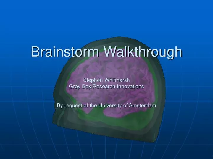
Brainstorm WalkthroughStephen WhitmarshGrey Box Research InnovationsBy request of the University of Amsterdam
Background • Brainstorm is software written in MATLAB for the analysis and visualization of MEG and EEG data. It provided routines for computing forward models based on spherical and realistic boundary element methods. These latter require that a tessellated representation of the brain, skull and scalp is provide for use in these calculations. Inverse methods include dipole fitting based on the MUSIC scanning method and cortically constrained minimum norm imaging. Also software is included for volumetric and surface rendering of inverse solutions. The methods implemented in this software are described in their publications, which can be accessed at http://neuroimage.usc.edu. They have provided a graphical user interface to their software, but all of the basic functions can be called from the command line and are documented at the BrainStorm website. • This walkthrough will make use of most visualization routines, using data from our own experiments at the UvA. For converting this EEG data into the Brainstorm format a simple Matlab routine is provided (BV2BS.mat) that can be found in the CNGGP folder on the local computer as well as on the UvA network (Bigbrother). For accurate localization of the custom EEG electrode positions of the experiment, measurements have been done by the Neuronav system and will be imported together with the EEG data. • This walkthrough will describe, in a step-by-step way, how to use Brainstorm for the following ends: • Projecting EEG activity on a 3D reconstruction of the cortex (together with layers of CSF, skull and scalp) • Source localization • Cortical bounded Minimal Norm imaging • For this purpose many steps have first to be done. These can become quite confusing since Brainstorm will launch many GUI’s, and the whole toolbox is still under construction (Beta). Please try to follow the instructions closely and feel free to ask for assistance at any moment. Additional information can be found in the Tutorial and Forum section of the Brainstorm website. One thing is clear though, that your efforts will pay of with impressive visualizations, only possible with this toolbox. • Enjoy!
Neurnav system recorded 3D locations of EEG sensors and fiducial points These will all be combined to permit localization of EEG activity on the MRI and 3D surfaces EEG recordings were made with a custom 32+16 channel cap From a high-resolution MRI scan 3D tessellated surfaces were made
Content • Creating Brainstorm study • Importing BVA EEG data and custom electrode locations • Aligning electrode locations to Subject Coordinate System (SCS) • Warping 3D surfaces and MRI scan to electrode locations • Projecting activity on 3D white matter surface • Aligning 3D surfaces to MR scan • Creating BEM head model • Minimal Norm Imaging of difference wave from masking experiment • Extracting signal from Minimal Norm • Creating 3Spheres (BERG) head model • Source localization of Myriam’s study
First study: Stack-Frame • We will start by working with data from a stack-frame paradigm. The ERP represents the additional activity (via a subtraction) correlatedwith boundary detection.
Importing EEG data • Startup brainstorm. Several windows will open. Notice the window called ‘Brainstorm – v…’ from which you can call all others.
Importing EEG data • Activate the Data Manager via File in the main window. • Open the Protocol window via Database new/edit protocols • Click new and select the appropriate directories (..\Tutorial\Data & ..\Tutorial\Subject) and press Save. • Do what the popup wants: Database New/Edit Subjects in Database • Fill in the fields by own preference and click add. • Be sure to put whatever name in front of ‘_brainstormsubject.mat’, default is the same of the subject, but leave the latter part unchanged for future reference.
Importing EEG data We are now ready to import the EEG dataset. • Data Manager Database New/Edit Datasets (EEG/MEG) Import New • Select the subject that has just been made in the right-side box and then select ‘raw format’ from the dropdown menu. • It will ask for a Study (i.o.w. the name of the experiment). Press cancel to make one. Name it e.g. ‘tutorial’ and click add,Save and Done. • Select the brainstormstudy file that has been created, then: • chLocations_32+16_Subject.txt voor Sensor Locations • CTF as coordinate system (we will get to the meaning of this soon) • Choose ‘Mixed: read file’ and select StackFrame_chType • (This will select certain channels as ‘bad’ that are only used as reference) • ‘Cancel’ for Orientations (only used for MEG) • StackFrame_chLabels.txt for Channel Labels • ‘Cancel’ for Reference Weights • StackFrame_data.raw for Spatio-temporal Data Matrix (EEG data) • StackFrame_sTiming for Time Values (sample times) • Yes to Transpose • Press Close • Select Main window Inverse Solutions Interactive. A new window ‘data viewer’ opens. Dont change anything yet but just press plot to to see the timeseries overlayed per electrode.
Alignments • For a correct correspondence between electrodepositions and a 3D surface or MR scan, electrodepositions as well as the target of the projection have to refer to the same coordinate system. Brainstorm needs everything in the CTF orientation:
Alignments • For reference purposes four landmark-points (fiducials) have been measured on the scalp of a test subject, using the Neuronav system. At the same time ‘dummy’ electrode positions were measures: The Nasion, Left and right pre-auricular as well as the Inion. They have not been loaded as EEG channels (automatically marked as ‘bad channels’) but will be used to determine the coordinate system of all the other electrodes. • For determining the coordinate system of our 3D surfaces we will have to add these positions (Nasion, Left & Right pre-auricular) manually. • For the MRI scan fiducials are already supplied although we will probably have to displace them a bit to create a good overlap with the 3D surfaces.
Aligning 3D surfaces We’ll start with aligning the 3D surfaces • Main window Tools Surface Manager. A new window will appear, showing the four layers from the montreal phantom in a list. Select them all and then choose Align from the Action drop-down menu. • Again, new windows will appear: a Surface and Channel Alignment Tool as well as an Envelope Viz. Choose Direct from the pop-up. Right pre-auricular Nasion
Aligning surfaces Note: You can rotate the surfaces by opening the Camera Toolbar in the Envelope Viz (View Camera Toolbar) and selecting the utmost left option (orbit camera). Click somewhere on the Envelope Viz and drag the mouse to rotate the camera angle. • Press Nasion and place the cursor above the nose, on the head (See previous slide). Press Nasion again to confirm. Repeat for the Left and Right pre-auricular. • When done, tick the CTF box and press Align Surfaces. • Every surface now loaded (WhiteMatter, CSF, Skull and Scalp) will be re-written with appropriate coordinates (filenames: *_CTF) and appear in the surface manager. • Press Quit in the Surface & Channels Alignment tool.
Aligning MR brain We will put the MRI scan in the same coordinate system by appointing the same fiducials. • Main menu Tools MRI tool. • MRI File Load Brainstorm Format. Choose the tutorial_subjectimage. A pretty brainscan will appear with fiducials already appointed. They still have to be defined, though: • Image Coordinates Define Fiducials. Select the appropriate fiducials and press Assign for all three. Then press Done. • First select the same Tutorial_subjectimage to save (and overwrite) and then select the same file to load again. • The MRI scan has to be linked to the subject. Go to Data Manager Database new/edit subject in database. Press Refresh, Update and check is everything is there. • Press Close.
Aligning Electrode positions Finally the electrodepositions will be referenced in CTF. • In the main Brainstorm window tick the box that says EEG at the left. • Press Load Channels in the Surface and Alignment tool (if you closed the window in the meantime, First go to Tools Surface Manager, select all four CTF surfaces and then select Align in the drop-down menu again). • Select the tutorial_channel.mat file. This file has been generated when the data was imported. Electrodes will appear as yellow dots in the Envelope Viz. • Tick the CTF box on. • Select Align Channels, answer No, and select the appropriate fiducials (all the way at the bottom of the list: ‘nasion’, ‘left’ and ‘right’ respectively). Note that most electrodes will still not appear on the scalp surface since the shape of the electrode-cap and the shape of the Phantom surface are different. For that purpose we will now ‘warp’ the Phantom surfaces, together with the accompanying MRI scan, to the electrode positions.
Warping • In the Alignment Tool press Phantom. • Answer No to remove channels – we need the ‘bad’ channels for a better fit to the scalp shape. • Answer Yes to alignment. • The topmost Autoassign button will associate electrode positions that have been loaded with the similarly named default positions defined by the Phantom. Press that one and see the red warping vectors (pin-needles) in the Envelope Viz appear.
Warping • Press Go and select the appropriate files IN THE TUTORIAL DIRECTORY! It points at the Montreal Phantom by default. • select Tutorial_4layer_tess.mat • Tutorial_subjectimage.mat • Wait until the message window tells you the new warped surfaces have been saved. • Open the surface manager again via the main window (tools) to refresh its content. • In the surface manager now deselect all surfaces that have been ticked in the view box. Select instead all four warped surfaces, tick the view box and press View. • (Tip: select one surface, press CTRL-A and then tock & un-tick the View box to deselect all surfaces). Rotate the 3D surface again to see that it now has a somewhat different shape then before. • In the actions drop-down menu select View Channels (and select the same channel file as before) to check if electrode positions now show up on the scalp surface.
Example • For some nice visuals: Select subsequently outer to inner layers (Scalp, Skull & CSF) in the surface manager and make them transparent with the slide on the left in the surface manager. You can also pick a separate color for each layer.
Checking alignment with MR We will now have to check if we succeeded aligning the 3D surface with the MRI image. • Open the MRI Tool and load the warped subjectimage (Main Window Tools MRI Tool MRI File Load Brainstorm format). You will notice a samewhat different shape MRI image. It is now warped to fit the electrodepositions and, in effect, will resemble the shape of the subject on which we recorder those electrode positions. • Overwrite the original subjectimage with this warped image (MRI File Save in Brainstorm format). Somehow if you don’t it will keep using the original one for the next calcualtions • Open or activate the surface manager window and select the warped white matter surface • From the action drop-down menu select check alignment with MRI. This can take a while (approx. 5 minutes). • The MRI viewer will appear and will show the warped tessellated surface in yellow on the MR scan. Work the slides to check the alignment. The process can be repeated for the other three surfaces (CTF, Skull and Scalp). Adjust the fiducials on the MRI scan if the alignment seems not good enough (selecting, defining and saving procedure as before). TIP: since we will be interested in the posterior part of the brain at least that alignment should be rather accurate. If the yellow boundaries show up too high with respect to the MRI, the fiducials of the MRI (left and right auricular) can be moved downwards. You can probably leave the nasion in its place. See the next slide as an example (I worked hard on that one, for now it doesn’t have to be perfect).
Some payoff now: Visualizing the data Now a simple but visually appealing presentation of the data can be made. • Make sure that warped 4 layer-tess is selected in the surface drop-down menu of the main Brainstorm window. • Refresh the Data Viewer window (Main Window Inverse Solution Interactive). • Now, in the data viewer window, select 3D Scalp Surface in the drop-down menu under Data viewing. • Press Plot, select white matter, and ‘do the twist’. • You can now add the other (warped) surfaces (select in the list, tick the view box and press the viewbutton). • Play around, if you want, with the transparency and camera angle. • In the time window in the data viewer a time-point or average over an interval (work with step) can be selected, which will be updated on the 3D surface projection. • With the truncate slide on the surface manager more or less signal can be shown. • Try pressing the go button next to smooth once or more while the white matter is selected in the surface manager. It is also possible to add curvature in grey. • Try walking through the timecourse (in Data Viewer press the arrow) and see what the signal does in the Envelope Viz!
Forward problem • Given a set of EEG signals from an array of external sensors, the inverse problem involves estimation of the properties of the current sources within the brain that produced these signals. Before we can make such an estimate, we must first solve the forward problem, in which we compute the scalp potentials and external fields for a specific set of neural current sources. The electric potential picked up by the EEG sensors has first traveled through the cerospinal fluid, the skull and scalp. These all have different characteristics of electric conductivity and will distort/spread the electric potentials differently before the signal is finally picked up by the EEG sensors. Methods for localizing electric fields (or magnetic as in MEG) can solve the forward problem in several ways. • One way is using simplified geometries so that the head is assumed to consist of a set of nested concentric homogeneous spherical shells representing brain, skull, and scalp. We will use this approach to localize dipoles within the brain. • Of course the brain, skull and scalp are in reality not spherical as well and are also anisotropic and inhomogeneous. More accurate solutions to the forward problem can use anatomical information obtained from high resolution volumetric brain images obtained with MR or CT imaging. We have already seen the 3D surfaces that were extracted from MR images. These can be included in the Boundary Element Method (BEM) for more accurate calculations. Although it uses realistic shapes, it still assumes homogeneity and isotropy within each region of the head. We will use the BEM method for Minimal Norm imaging. This assumes that primary sources are currents in the cortical surface. Thus a current dipole is assigned to each of many tens of thousands of tessellation elements perpendicular to cortical surface. The Minimal Norm image will try to create a least-squares solution using the least amount of (cortical) dipoles.
3 Spheres Headmodel We will start with the 3 Spheres Headmodel • Tools Headmodel Advanced. • Select 3 Shell-Sphere (BERG) in the forward modeling box. • In the head compartments select the warped scalp and the warped white matter for the scalp and cortex respectively. Tick the Compute in the Volume Source Grid box. • Press Adjust in the Sphere Parameters box to see the fitted spheres on the scalp in the Envelope Viz. See Example. • You can adjust the sphere parameters, but for now leave them at default value. • Tick the Compute box under Volume Source Grid. • Press Run • The headmodel will be saved in the Data folder and appear in the main Brainstorm window under the Headmodel drop-down menu. A way to make this spherical headmodel more realistic it to first warp the MRI scan and 3D surfaces to a sphere. Since MEG electrodes are positioned in a sphere anyway, using this approach with MEG sensors will be feasible.
Updating • It could happen that Brainstorm does not update all the available files (e.g. headmodel). • Go to Data Manager Database new/edit subject in database. Press Refresh and then Update and check is everything is there.
RAP-MUSIC Brainstorm’s source localization method is called RAP-MUSIC. MUSIC stands for Multiple Signal Classification Approach. It can be applied for the whole time range thus creating fixed locations of dipoles, as well as for different time-epochs for which different solutions can be found. Because of the many possible number of sources located (equal to the number of sensors), Brainstorm uses the Recursively Applied and Projected (RAP) method. By this way after each successive source is found its contribution to the signal will be ‘projected away’, leaving the next source to explain the remaining signal. Moreover, one can specify the number of components that the search will start with, according to a manual selection of the number of components that the data will extract. • Open the Data Viewer window again (Inverse Solutions Interactive) • In the Analysis box select RAP-MUSIC. • The signal will be decomposed in several components. Slide through a number of ‘Ranks’ to see the re-composed signal when only several components are included in the further analysis. See next slide for an example.
Example Decomposed signal Unexplained signal number of components
RAP-MUSIC • Eventually select the suggested number of five or six components/dipoles you want to search forand press Done. They will subsequently be checked to the correlation threshold, and - if found - appear in the MRI tool window. • In the now appearing Parameters RAP-MUSIC choose: • Correlation Threshold on .85 • TruncatedCondition as Regularization, Parameter on 10. • Press Execute
RAP-MUSIC • It can happen that the computation stops and the Matlab interface appears. In that case it will ask you if you really want to continue while sources localized will not meet the statistical threshold. IF you want you can press continue (the downward arrow in the main toolbar of Matlab). • Click on the second source from the list (2) in the MRI Viewer. As can be seen in the Data Time Series Figure, the second source accommodates the second peak in the data and is placed more anterior to the first. How would you interpret these results?
Bug • Brainstorm needs some workarounds since it’s still in a Beta state. • Before calculating another headmodel the old one has to be removed. Take your Windows Explorer to the EEG folder of your subject and delete all headmodel files. The files all start with headmodel_*.
BEM Headmodel Next up is the BEM headmodel. We will use this to look at cortical sources of recurrent processing from a masking study with which you will be familiar now. • Tools Headmodeling Advanced • Select BEM in the second drop-down menu. • In the BEM parameters menu, select successively the Warped CSF, Skull and Scalp surfaces. In that order! You can view the surfaces by pressing view envelopes. • Change the Test method to Collocation for calculation speed (or else it will take hours). • In the Head Modeling Tool window select the warped white matter as Cortex under Head Compartments. That will be the source of the forward solution. • Press Run. When the message window says: ‘BEM with linear basis’ you will probably have to wait for a while (approx. 5 minutes).
BEM Headmodel The aligned surfaces for the BEM computation that will show up automatically should look something like this:
Masking Experiment • The results of the masking experiment have already been discussed in a previous practice. Summing up, re-entrant activity of the primary visual area’s is suppressed when a stimulus is shortly followed by a mask. This is shown by an absence of activity in the primary visual area’s between approx. 110 and 140 ms. For the purpose of localizing the ‘origin of the difference’ between masked and not-masked stimuli, the ERP from the masked stimuli is subtracted from the ERP from unmasked stimuli. See the next two slides to get an impression about the resulting difference wave from masked and unmasked stimuli. Try to formulate how the difference wave would look.
Importing EEG data We will now to import the data from the masking experiment in the same way as we sis before. • Data Manager Database New/Edit Datasets (EEG/MEG) Import New • Select the subject in the right-side box and then select ‘raw format’ from the dropdown menu. • Select the brainstormstudy file, then: • chLocations_32+16_Subject.txt voor Sensor Locations • CTF as coordinate system (we will get to the meaning of this soon) • Choose ‘Mixed: read file’ and select MaskNoMask_chType • (This will select those channels as ‘bad’ that are only used as reference) • ‘Cancel’ for Orientations (only used for MEG) • MaskNoMask_chLabels.txt for Channel Labels • ‘Cancel’ for Reference Weights • MaskNoMask_data.raw for Spatio-temporal Data Matrix (EEG data) • MaskNoMask_sTiming for Time Values (sample times) • Yes to Transpose • Press Close • Select Main window Inverse Solutions Interactive. A new window ‘data viewer’ opens. Dont change anything yet but just press plot to to see the timeseries overlayed per electrode.
Minimal Norm Imaging • Close the Surface Manager, the Envelope Viz and in Data Manager press refresh. • Make sure the warped MRI and warped 4 layer tess surfaces are selected in the Main BrainStorm window. • In the Main BrainStorm window the headmodel should also have appeared. • Via the Main BrainStorm window go to Inverse Solutions Interactive. • In the analysis section choose Minimal Norm imaging in the drop-down menu of the Source Imaging box. • We’ll constrain the solution a bit by adjusting the Tikonov regularisation to 50%. • We’ll calculate the Minimal Norm for every timepoint so we can see it evolve over time. The time-course interval for which the Minimal Norm will be calculated is taken from the data-viewer box and although it can be adjusted here, for the moment just press go.
Minimal Norm Imaging • The minimal norm image will shown on the 3D warped cortical surface in a new Envelope Viz. • Scroll through the time-course in the Data Viewer and see the Minimal Norm solution for that timecourse displayed in the Envelope Viz. • We can now look up the moment in time at which the difference wave will show re-entrant processing at the occipital pole. Scroll to 110 ms. It should look something like this:
Minimal Norm Imaging We are now able to extract mean signal from the dipoles. • First make sure the MRI Manager window is open. If not do so and load the warped subjectimage. • Go to the surface manager and in the action drop-down menu select Dispatch Scouts. • Press probe on the now appearing Cortical Scout Manager and move along the 3D white matter surface. Notice that the location of the crosshairs will be projected on the MRI scan. • Click on the most activated area (e.g. left occipital pole) We will include several vertices (each containing a dipole). • Tick the constrained box in the Cortical Scout Manager. This will result in only selecting those vertices that are ‘active’ according to the colored overlay. • Press ‘+’ next to scout size in the Cortical Scout Manager a couple of times to enlarge the probed area. See the next slide for an example. Also notice that the location of the probe is shown on the MRI scan. • Deselect the Absolute values box in the Cortical Scout Manager for a more appealing comparison with the original EEG data. • Press Activate on the Cortical Scout Manager to extract the Mean time series. • You can add more scouts and by selecting them together, can overlay the activity (see next slide for an example).
Concluding this part… • Do you see the data -as is has been visualized now- confirm the hypothesis of interrupted re-entrant processing by masking?
That’s it! • Please feel free to play around now. (BrainStorm is freeware)