Download
1 / 20
210 likes | 412 Vues
Introduction to algorithmic models of music cognition. David Meredith Aalborg University. Algorithmic models of music cognition. Most recent theories of music cognition have been rule systems, algorithms or computer programs

E N D
Introduction to algorithmic models of music cognition David Meredith Aalborg University
Algorithmic models of music cognition • Most recent theories of music cognition have been rule systems, algorithms or computer programs • Take representation of musical passage as input and output a structural description • Structural description should correctly describe aspects of how a listener interprets the passage
Algorithmic models of music cognition • Models take different types of input • audio signals representing sound • representations of notated scores • piano-roll representations • Type of input depends on purpose of model
Algorithmic models of music cognition • A structural description represents a listener’s interpretation – so cannot be tested directly • Need to hypothesise how the listener’s interpretation will influence his or her behaviour
Longuet-Higgins’ model (1976) • Computer program that takes a performance of a melody as input and predicts key, pitch names, metre, notated note durations and onsets, phrasing and articulation OUTPUT: [[[24 C STC] [[-5 G STC] [0 G STC]]] [[1 AB] [-1 G TEN]]] [[[REST] [4 B STC]] [1 C TEN]]
Longuet-Higgins’ model (1976) • Uses score as a ground truth • Assumes pitch names, metre, phrasing, key, etc. should be as notated in an authoritative score of the passage performed • Note fourth note here spelt as an Ab not a G# OUTPUT: [[[24 C STC] [[-5 G STC] [0 G STC]]] [[1 AB] [-1 G TEN]]] [[[REST] [4 B STC]] [1 C TEN]]
Longuet-Higgins’ model (1976) • Even calculating notated duration and onset of each note is not trivial because performed durations and onsets will not correspond exactly to those in the score • e.g., need to decide whether timing difference is due to tempo change or change in notated value OUTPUT: [[[24 C STC] [[-5 G STC] [0 G STC]]] [[1 AB] [-1 G TEN]]] [[[REST] [4 B STC]] [1 C TEN]]
Longuet-Higgins’ model (1976) • Program assumes that perception of rhythm is independent of perception of tonality • So rhythm perceived not affected by pitch • actually not strictly true (cf. compound melody) • Assumes metre independent of dynamics • can perceive metre on harpsichord and organ where dynamics not controlled • Only considers metres in which beats within a single level are equally-spaced • One or two equally-spaced beats between consecutive beats at the next higher level OUTPUT: [[[24 C STC] [[-5 G STC] [0 G STC]]] [[1 AB] [-1 G TEN]]] [[[REST] [4 B STC]] [1 C TEN]]
Longuet-Higgins’ model of rhythm • To start, listener assumes binary metre • Changes interpretation if given enough evidence • current metre implies a syncopation • current metre implies excessive change in tempo • If enough evidence, then changes to a metre where no syncopation and/or smaller change in tempo implied
Longuet-Higgins’ model of tonality • Estimates value of sharpness of each note • i.e., position on line of fifths • Theory has six rules • First rule says that notes should be spelt so they are as close as possible to the tonic on the line of fifths • Other rules control how algorithm deals with chromatic intervals and modulations • e.g., second rule says that if current key implies two consecutive chromatic intervals, then change key so that both become diatonic
Longuet-Higgins’ model: Output • Section of coranglais solo from Act III of Wagner’s Tristan und Isolde • Triplets in first beat of fifth bar • Grace note in seventh bar • Output agrees with original score here • In a larger study (Meredith 2006, 2007) LH’s model correctly predicts 98.21% of pitch names in a 195972 note corpus • cf. 99.44% spelt correctly by Meredith’s PS13s1 algorithm
Lerdahl and Jackendoff’s (1983) Generative Theory of Tonal Music (GTTM) • Probably the most influential and frequently-cited theory in music cognition • Takes a musical surface as input and produces a structural description that predicts aspects of an expert listener’s interpretation • not entirely clear what information assumed in input • predicts “final state” of listener’s interpretation – not “real-time” experience of listening
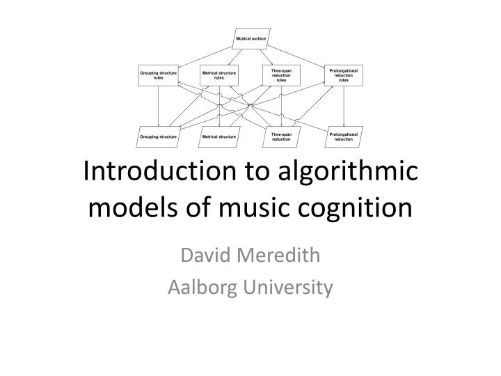
GTTM • Four interacting modules • Grouping structure: motives, themes, phrases, sections • Metrical structure: “hierarchical pattern of beats” • Time-span reduction: how some events elaborate or depend on other events • Prolongational reduction: the “ebb-and-flow of tension”
GTTM • Each module contains two types of rule • Well-formedness rules: define a class of possible analyses • Preference rules: isolate best well-formed analyses • Modules depend on each other (sometimes circularly!) • Metre requires grouping • Grouping requires time-span reduction • Time-span reduction requires metre • Therefore not trivial to implement the theory computationally • Though some have tried (e.g., Temperley (2001), Hamanakaet al. (2005, 2007))
Temperley and Sleator’sMelisma system • Temperley (2001) presents a computational theory of music cognition, deeply influenced by GTTM • see Meredith (2002) for a detailed review • Uses well-formedness rules and preference rules like GTTM • Models six aspects of musical structure • metre • phrasing • contrapuntal structure • pitch-spelling • harmonic structure • key-structure
Melisma • Consists of five programs that should be piped as shown at left • Evaluated output by comparison with scores • 46 excerpts from a harmony text book (Kostka and Payne, 1995, 1995b)
Melisma • Input in the form of a note-list or piano-roll giving onset time, duration and MIDI note number of each note • Must first infer metre using meter program • But harmony can influence metre and vice-versa, so should use a “two-pass” method as shown • The notelist and beatlist are then given as input to the other programs
Using Temperley’s model to explain listening, composition, performance and style • Melisma programs scan music from left to right, keeping note of the analyses that best satisfy the preference rules at each point • Ambiguity: Two or more best analyses at a given point • Revision: The best analysis at a given point is not part of the best analysis at a later point • Expectation: We most expect events that lead to an analysis that doesn’t conflict with the preference rules • Style: A piece is in the style of the preference rules if it satisfies them not too well (boring) and does not conflict with them too much (incomprehensible) • Composition: Compose a piece that optimally satisfies the preference rules • Performance: Temporal and dynamic expression aimed at conveying structure that best satisfies the preference rules
Summary • Can model music cognition using algorithms that generate structural descriptions from musical surfaces • We can evaluate such algorithms by comparing their output with expert analyses and authoritative scores • Some well-developed theories of music cognition take the form of preference-rule systems containing • Well-formedness rules that define a class of legal analyses • Preference rules that identify the well-formed analyses that best describe the listener’s experience
References • Hamanaka, M., Hirata, K. & Tojo, S. (2005). ATTA: Automatic time-span tree analyzer based on extended GTTM. Proceedings of the Sixth International Conference on Music Information Retrieval (ISMIR 2005), London. pp. 358—365. http://ismir2005.ismir.net/proceedings/1015.pdf • Hamanaka, M., Hirata, K. & Tojo, S. (2007). ATTA: Implementing GTTM on a computer. Proceedings of the Eighth International Conference on Music Information Retrieval (ISMIR 2007), Vienna. pp. 285-286. http://ismir2007.ismir.net/proceedings/ISMIR2007_p285_hamanaka.pdf • Kostka, S. & Payne, D. (1995a). Tonal Harmony. New York: McGraw-Hill. • Kostka, S. & Payne, D. (1995b). Workbook for Tonal Harmony. New York: McGraw-Hill. • Lerdahl, F. and Jackendoff, R. (1983). A Generative Theory of Tonal Music. MIT Press, Cambridge, MA. • Longuet-Higgins, H. C. (1976). The perception of melodies. Nature, 263(5579), 646-653. • Longuet-Higgins, H. C. (1987). The perception of melodies. In H. C. Longuet-Higgins (ed.), Mental Processes: Studies in Cognitive Science, pp. 105-129. British Psychological Society/MIT Press, London/Cambridge, MA. • Meredith, D. (2002). Review of David Temperley’sThe Cognition of Basic Musical Structures (Cambridge, MA: MIT Press, 2001). Musicae Scientiae, 6(2), pp. 287-302. • Meredith, D. (2006). The ps13 pitch spelling algorithm. Journal of New Music Research, 35(2), pp. 121-159. http://taylorandfrancis.metapress.com/link.asp?id=q679l61r31m18460 • Meredith, D. (2007). Computing Pitch Names in Tonal Music: A Comparative Analysis of Pitch Spelling Algorithms. D. Phil. dissertation. Faculty of Music, University of Oxford. http://www.titanmusic.com/papers/public/meredith-dphil-final.pdf • Temperley, D. (2001). The Cognition of Basic Musical Structures. MIT Press, Cambridge, MA.