Download
1 / 45
450 likes | 643 Vues
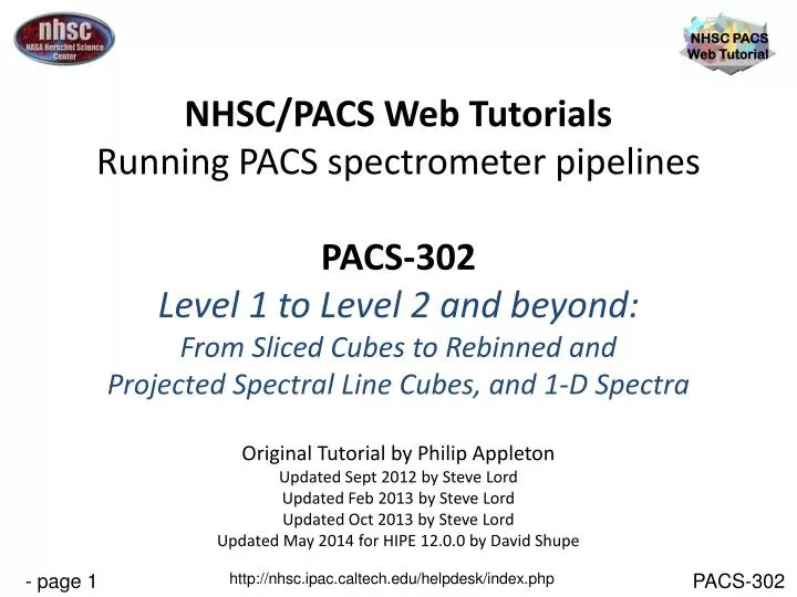
NHSC/PACS Web Tutorials Running PACS spectrometer pipelines PACS-302 Level 1 to Level 2 and beyond: From Sliced Cubes to Rebinned and Projected Spectral Line Cubes, and 1-D Spectra Original Tutorial by Philip Appleton Updated Sept 2012 by Steve Lord Updated Feb 2013 by Steve Lord

E N D
NHSC/PACS Web Tutorials Running PACS spectrometer pipelines PACS-302 Level 1 to Level 2 and beyond: From Sliced Cubes to Rebinned and Projected Spectral Line Cubes, and 1-D Spectra Original Tutorial by Philip Appleton Updated Sept 2012 by Steve Lord Updated Feb 2013 by Steve Lord Updated Oct 2013 by Steve Lord Updated May 2014 for HIPE 12.0.0 by David Shupe
Introduction This tutorial presents the main steps of the standard pipeline starting from the calibrated Frames (Level 1) and pacsCube (also Level 1). It describes the processing steps needed to create a set of Pacs “Rebinned Cubes “ and (especially if the observation is a raster) a Projected Cube. Numerous break points are shown, where one can interactively examine the intermediate results of the pipeline. The PACS Spectroscopy pipelines are documented here: PACS Data Reduction Guide: Spectroscopy, e.g., Chapter 3 These documents can be access through the HIPE help pages.
Important additional material for each release is found online at the PACS public Twiki: http://herschel.esac.esa.int/twiki/bin/view/Public/PacsCalibrationWeb Also, find out what is new for pipeline 12 here: http://herschel.esac.esa.int/twiki/bin/view/Public/HipeWhatsNew12x#Pipeline
Tutorial Pre-requisites: • HIPE is running version 12.0 (or user build 11.0.2603) or later • You have completed the following tutorial:. • PACS-301 PACS Spectroscopy Level 0 to 1 Processing
At this point in the processing we had just completed the last step of tutorial PACS 301. We last performed the flat field step after having created a set of sliced Cubes (step 3 below). We also did some cleanup (steps 4 & 5 below) In this tutorial we continue working with obsId = 1342186799 camera = blue Our last steps which brought us to Level 1:
Let’s recap the structure of the data products so far, and see where we are going: Level 0 -1, and Level 2 Products PACS PIPELINE CUBE BUILDING SINGS background FRAMES RAW Level 0 To Level 0.5 Projected to 3” x 3” pixels To calibrated L1 FRAMES CALIBRATED PACSCUBE REBINNED PROJECTED FRAMES CUBE CUBE CUBE Level 1 Level 2
Let’s recap the structure of the data products so far, and see where we are going: Near the end of the Level 1 pipeline, we created a set of pacsCubes. There are 4 pacsCubes in our example, because this blue AOR contains4 slices (Nod A and Nod B for each of two different lines) PACS PIPELINE CUBE BUILDING SINGS background FRAMES RAW Level 0 To Level 0.5 Projected to 3” x 3” pixels To calibrated L1 FRAMES CALIBRATED PACSCUBE REBINNED PROJECTED FRAMES CUBE CUBE CUBE Level 1 Level 2
Level 1 to 2 overview: Step 1 Check number of Frame and Cube Slices from level 1 Step 2 Create a wavelength grid for binning Step 3 Flag data with user-controlled sigma-clipping Step 4 Create the rebinned cube and average the NODS Step 5 Inspect the Rebinned Cube Spaxel-by-Spaxel Step 6 (for Raster or dither pattern mapping of extended sources) Project Rebinned Cubes (via specProject or Drizzling) onto a WCS Step 6 (for point sources and single pointings) Extract spectra from the central pixel Step 7 Explore Rebinned and Projected cubes in Spectrum Explorer
Step 1 Check that you have converted your frames to pacsCubes (5 x 5 x N) product, and that you have the correct number of both
A pacsCube is simply a reorganized Frame with dimensions which are 5 x 5 x Nwhere the 5 x 5 refers to the IFU spaxels of PACS, and N is the number of time samples which translate into grating position and wavelength. In a senseyou can think of the pacsCube as a spatial representation of sky (5 x 5) and the third dimension can be translated into wavelength—forming the basic dataset or “cloud of wavelength samples” as a function of position. In our example we had 4 slices of Frames. Now, having executed the last step, we have 4 slices of Cubes. These slicedCube and slicedFrame entities (objects) are simply collections of Frames and Cubes sliced by raster position (if relevant), Nod position (Nod A and B) and Line ID. In this case we have two lines each with two Nod observations. Had we done not one, but “n” repetitions of the Nod cycle, we would 2n separate nods for each line. Since this was a simple pointed observation with one repetition, we have only 4 slices of both frames and now, as of the last step, 4 cubes
Check One—Lets look to check that we have the correct number of level1 Frames and pacsCubes Type into the Console window the following slicedSummary(slicedFrames) slicedSummary(slicedCubes)
Summary of Level 1 Products HIPE> slicedSummary(slicedFrames) noSlices: 4 noCalSlices: 0 noScienceSlices: 4 slice# isScience nodPosition nodCycle rasterId lineId band dimensions wavelengths 0 true ["B"] 1 0 0 [2] ["B3A"] [18,25,960] 63.093 - 63.379 1 true ["A"] 1 0 0 [2] ["B3A"] [18,25,960] 63.093 - 63.379 2 true ["B"] 1 0 0 [3] ["B3A"] [18,25,960] 57.213 - 57.548 3 true ["A"] 1 0 0 [3] ["B3A"] [18,25,960] 57.213 - 57.548 Above are 4 Frames (18x25x960) representing 1+16+1 (=18) spectral pixels, 25 spatial pixels (the 5 x 5 array) and 960 time samples. Note the 16 spectral pix plus 2 extra (a “open” channel and an “overscan”) making 18 spectral pixels total HIPE> slicedSummary(slicedCubes) noSlices: 4 noCalSlices: 0 noScienceSlices: 4 slice# isScience nodPosition nodCycle rasterId lineId band dimensions wavelengths 0 true ["B"] 1 0 0 [2] ["B3A"] [15360,5,5] 63.093 - 63.379 1 true ["A"] 1 0 0 [2] ["B3A"] [15360,5,5] 63.093 - 63.379 2 true ["B"] 1 0 0 [3] ["B3A"] [15360,5,5] 57.213 - 57.548 3 true ["A"] 1 0 0 [3] ["B3A"] [15360,5,5] 57.213 - 57.548 HIPE> After conversion to slicedCube we now have 4 pacsCubes, organized as time sample*16 (=15360), 5 x 5 in this case. Note that the open and overscan spectral pixels have been stripped off in the pacsCube format.
Step 2 Create a wavelength grid. This will be used to grid the spectrum in “wavelength-space” and is the first step in constructing a re-binned cube. In the default case the grid is Nyquist-sampled. However, the user can select a finer grid or, alternatively, a courser grid to effectively provide additional smoothing.
Creating a wavegrid: the grid resolution and number of phased samplings are governed by the parameters “oversample” and “upsample”, respectively. The default values of these are oversample = 2, upsample = 1. The default values provide a grid which oversamples the intrinsic spectral resolution element by a factor of 2 (i.e., Nyquist sampling). An upsample value of 1 means that one contiguous set of wavelength bins are laid-out. When oversample is “m”, the binwidth used is the intrinsic resolution element/m. When upsample is “n”, n sets of wavlength bins are laid-out, each phased by the binwidth/n.waveGrid=wavelengthGrid(slicedCubes.refs[0].product, oversample=2, upsample=1, calTree = calTree)Illustrative examples follow….
Examples of Oversample and Upsample Parameter Pairs
Oversample = 2 Upsample = 1 bins = ½ spectral resolution at that wavelength spectral resolution = 0.02mm BINS widths are ½ the spectral resolution element = Nyquist Sampled SAMPLES TAKEN HERE
Oversample = 4, Upsample = 1 bins = 1/4 spectral resolution at that wavelength Oversample = 4 means 4 times narrower bins that the spectral resolution (2 x better than Nyquist) spectral resolution = 0.02mm
Oversample = 2 Upsample = 2 bins = ½ spectral resolution at that wavelength, but bins are shifted by ½ a bin and resampled, thus the final spectrum contains a finer grid (although the values are not independent). Sample with oversample = 2 (oversample = 2) then shift by ½ bin then sample again (upsample = 2) BINS are ½ spectral resolution = Nyquist Sampled spectral resolution = 0.02mm
Oversample = 2, Upsample = 3 ; Binwidths are ½ the spectral resolution at their wavelength, and bins are shifted by 1/3 and 2/3 of a binwidth and resampled. Thus, the final spectrum contains a fine-spaced grid, but one with highly correlated samples. BINS are ½ spectral resolution = Nyquist Sampled spectral resolution = 0.02mm Sample with oversample = 2 (oversample = 2) then shift by 1/3 bin then sample again (upsample = 3 Sample centers are spaced at intervals 1/3 the binwidth.
Step 3 Before regridding, we apply OUTLIERS rejection flagging to the spectra. This process is quite robust and is found to work well for PACS spectra. If the user suspects that the Deglitcher is over-flagging with GLITCH flags, the effect of these GLITCH flags can be turned-off and the de-glitching can instead be done with the OUTLIERS rejection flag method
Next we active the masks and applya sigma-clipping routine to the spectra(See PACS Data Reduction Guide: Spectroscopy, 3.3.8. for details) # Activate all masks slicedCubes = activateMasks(slicedCubes, String1d([str(i) for i in slicedCubes.get(0).maskTypes\ if i not in ["INLINE", "OUTLIERS_B4FF"]]), exclusive = True) # Flag the remaining outliers, (sigma-clipping in wavelength domain) slicedCubes = specFlagOutliers(slicedCubes, waveGrid, nSigma=5, nIter=1) specFlagOutliers has the task of defining a new flag called “OUTLIERS” created using a simple sigma-clip algorithm on each bin. nIter=1 means that the algorithm has been applied once and then again, iteratively rejecting points > nSigma. The user can experiment with these two parameters. The output of this routine is to create a mask. The mask is later applied when the actual rebinning of the spectra onto the waveGrid takes place. The mask is called “OUTLIERS” and is activated in the next step. NOTE ON EXCLUSION OF GLITCH MASK: If you choose to exclude the glitch detection from your results, remove the “GLITCH” string from the activateMasks command above. This will ignore the glitch mask. We have had good results by doing this.
Now we will create our first set of rebinned cubes—one for each pacsCube (in our lineId=2 case, we have two—one for Nod A and one for Nod B) PACS PIPELINE CUBE BUILDING SINGS background FRAMES RAW Level 0 To Level 0.5 Projected to 3” x 3” pixels To calibrated L1 FRAMES CALIBRATED PACSCUBE REBINNED PROJECTED FRAME CUBE CUBE CUBE Level 1 Level 2
Step 4 Create the Rebinned Cube of dimensions 5 x 5 x rebinned wavelength elements
Now Create the Rebinned Cube We activate the OUTLIER mask for the first time. This happens before rebinning # Activate all masks slicedCubes = activateMasks(slicedCubes, String1d([str(i) for i in slicedCubes.get(0).maskTypes\ if i not in ["INLINE", "OUTLIERS_B4FF"]]), exclusive = True) # Rebin all selected cubes on the same wavelength (mandatory for specAddNod) slicedRebinnedCubes = specWaveRebin(slicedCubes, waveGrid) This step produces a set of rebinned cubes (one slice per cube) NOTE ON EXCLUSION OF GLITCH MASK: If you choose to exclude the glitch detection from your results, add the “GLITCH” string to the activateMasks command above. This will ignore the glitch mask. We have had good results by doing this. This is the second and last time you need to worry about ignoring the glitch mask. If you performed this step and the one before specFlagOutliers then you will have a rebinned cube which excludes the glitch detection and relies on the sigmaClipping for removal of outliers. In general, we have found sigmaClipping to produce the better results.
Step 4 (con’t) Average the Nods
Now we average together the two Nod positions. For an observation with a set of raster positions, there will still be more than one final cube (store as slices)—one for each raster position # Average the nod-A & nod-B rebinned cubes. # All cubes at the same raster position are averaged. # This is the final science-grade product currently possible, for all observations except # the spatially oversampled raster observations slicedFinalCubes = specAddNodCubes(slicedRebinnedCubes)
Step 5 Inspect the rebinned spectra—spaxel by spaxel using various diagnostic tools
With the verbose=1 diagnostics, we can view the central pixel (e.g.) profile along with the its estimated rms of line and continuum flux. Draw a box to zoom
Here we plot only the first slice. In the case we have set the lineId=2, so we have only the [OI] line. In the case of a raster observation, you can plot the profiles for each slice separately.
You can also extract a spectrum (in this case the central one: [2,2] ) and create a Spectrum1dproduct # Optional: extract the central spaxel of one slice into a simple spectrum # You can do this for any spaxel X and Y and any slice. It creates a # Spectrum1d class of product, on which various viewers will work slice = 0 spaxelX, spaxelY = 2,2 centralSpectrum = extractSpaxelSpectrum (slicedRebinnedCubes, slice=slice, spaxelX=spaxelX, spaxelY=spaxelY) On the next page we show how this can be studied in the variable list so that you can write to FITS or open in SpectrumExplorer.
You have reached LEVEL 2for a Single Pointed Observation Spectrum Explorer FITS In the variable list right-mouse click on CentralSpectrum and either “open with” the spectrum in Spectrum Explorer or send to a FITS file
Step 6 (for Raster Observations of Extended Sources) In order to mosaic your cubes onto a uniform World Coordinate System (WCS) grid, users with raster observations* should select between the two methods of mosaicking: you may using the superior method called “Drizzling”, which is also by far the more computer intensive method, or the alternative method, called “specProject” The methods project onto a 3” grid by default. *As opposed to the single-pointing example data set of this tutorial
The projected cube is only recommended for rasterobservation where you have many rebinned cubesand these are combined into a final projected cube PACS PIPELINE CUBE BUILDING SINGS background FRAMES RAW Level 0 To Level 0.5 Projected to 3” x 3” pixels To calibrated L1 FRAMES CALIBRATED PACSCUBE REBINNED PROJECTED FRAME CUBE CUBE CUBE Level 1 Level 2
specProject (Refer to section 3.7 of the “PACS Data Reduction Guide for Spectroscopy”) For it relative speed, specProject is recommended for large wavelength range observations and SEDS. Each output spaxel is formed from a weighted combination of overlapping and/or undersampled spaxels from the slicedFinalCubes (which have been rebinned in wavelength) for each spatial and wavelength point onto a (default) 3” grid.
Invoking specProject # specProject works on the final rebinned cubes. slicedProjectedCubes = specProject(slicedFinalCubes,outputPixelsize=3.0) # Display the projected cube in the Spectrum Explorer if verbose: slice = 0 oneProjectedSlice = slicedProjectedCubes.refs[slice].product openVariable("oneProjectedSlice", "Spectrum Explorer") The present script makes a slicedProjectedCube and even opens up a slice in Spectrum Explorer. Also available are other viewers (via right-mouse clicking on the variable “slicedProjectedCube”) as well as the same FITS writing capability as before.
Drizzling The Drizzling projection is so-named because the total “drops” of emission collected within input pixels are broken into smaller “droplets” to be collected and weighted into the output pixels. It differs from spacProject in that it operates on the Level 1 slicedPacsCubes prior to wavelength rebinning (not Level 2 cubes) and also differs in the inputs it takes when using the unchopped or chopped AORS. The ChopNodLineScan.py script includes both the Drizzle and specProject methods. (Primary drizzle document: http://www.stsci.edu/ftp/science/hdf/combination/drizzle.html)
Invoking Drizzling (slicedDrizzled Cubes)For parameter details, refer to section 3.7 of the PACS Data Reduction Guide (Spectroscopy) # Drizzling works from the not-rebinned cubes oversampleWave = 2 upsampleWave = 3 waveGrid = wavelengthGrid(slicedCubes, oversample=oversampleWave, upsample=upsampleWave, calTree = calTree) oversampleSpace = 3 upsampleSpace = 2 pixFrac = 0.6 spaceGrid = spatialGrid(slicedCubes, wavelengthGrid=waveGrid, oversample=oversampleSpace, upsample=upsampleSpace, pixfrac=pixFrac, calTree=calTree) slicedDrizzledCubes= drizzle(slicedCubes, wavelengthGrid=waveGrid, spatialGrid=spaceGrid)[0] These Drizzled Cubes may be viewed in Spectrum Explorer as well.
Invoking Drizzling (WARNING) Warning: In Pipeline 12 – DRIZZLING is run by default – that is – the drizzling script lines shown in the previous slide are not commented-out. The user should be sure that he/she wants to run drizzle before invoking it. The drizzle routine is an excellent optimized and powerful projection method (when sufficient oversampling has been obtained within the observation) but it can require many hours of execution time and large amounts of computer memory, especially for large maps or line ranges. It is best run on a large and perhaps remote virtual machine (via a VNC session) and utilizing multi-threading. The user’s alternative, specProject will, in general, yield a fairly good projected map in much shorter processing times.
Step 6 (for point sources and single pointings) Extract spectra forthe central spaxel
Making a projected cube (using specProject or Drizzling) from a single pointing is not recommended, but it is also not prohibited. However, the formal final product from a single pointing is considered to be a rebinned cube, not any projected cube. One may attempt to project a single pointing for visualization purposes (such as is done in this tutorial), but, because the PACS IFU footprints are distorted, flux conservation is typically not maintained in the output map. Only in the case of a fully sampled raster (spatial dithered mapping) can one expect to recover proper fluxes from a projected cube. Caveat: Making a projected cube from a single pointing
Correcting and Extracting Point Sources Caveats: The instructions following assume that the user has employed a single pointing for a target that is a point source*, and the target’s photocenter is somewhere within the central spaxel [2,2] (i.e., the flux peaks at spaxel [2,2])**. *If there are multiple pointings, these should be handled separately as per the instructions below using the individual rebinned cubes. (The PACS point source corrections operate only on individual rebinned cubes.) **If the source is in a spaxel other than the central spaxel, use “PACS Point Source Loss Correction” script found in HIPE->Scripts->PACS useful scripts. • extractCentralSpectrum will return three spectra: • Spectrum of the central pixel corrected for the part of the beam that the central spaxel misses. This is known as the c1 spectrum. • Spectrum of the sum of the central 9 pixels, with the (much smaller) correction for the part of the beam that this “superspaxel” misses: the c9 spectrum. • c) Spectrum of the central pixel, with the “3x3” correction that compares the ratio of c1 to c9 to the ratio expected from the beam profile; this is intended to correct for small mis-pointings and is the c129 spectrum (‘c one-to-nine’, get it?). To trust this correction the source continuum must be of order 10 Jy. • Discussions of these corrections are found in the PACS Data Reduction Guide: Spectroscopy section 3.7.3.
Extracting the central spaxel and returningthree spectra with various corrections for slice in range(len(slicedFinalCubes.refs)): if verbose: print # a. Extract central spectrum, incl. point source correction (c1) # b. Extract SUM(central_3x3 spaxels), incl. point source correction (c9) # c. Scale central spaxel to the level of the central_3x3 (c129 -> See PDRG & print extractCentralSpectrum.__doc__) c1,c9,c129 = extractCentralSpectrum(slicedFinalCubes, slice=slice, smoothing='median', isLineScan=-1, calTree=calTree, verbose=verbose) # # Save to Fits if saveOutput: name = nameBasis + "_centralSpaxel_PointSourceCorrected_Corrected3x3NO_slice_" simpleFitsWriter(product=c1,file = outputDir + name + str(slice).zfill(2)+".fits") name = nameBasis + "_central9Spaxels_PointSourceCorrected_slice_" simpleFitsWriter(product=c9,file = outputDir + name + str(slice).zfill(2)+".fits") name = nameBasis + "_centralSpaxel_PointSourceCorrected_Corrected3x3YES_slice_" simpleFitsWriter(product=c129,file = outputDir + name + str(slice).zfill(2)+".fits") Some plots are produced but are not shown here. Since the example in this tutorial is not a point source, the plots are not helpful to discuss at this point.
Step 7 Explore your final projected or rebinned cube with the Spectrum Explorer, or your favorite viewer, or to make spectral maps.
The Spectrum Explorer provides many visualization options as well as line fitting You may display and examine the final spectral cubes with the Spectrum Explorer. Further processing can be conducted there using, e.g., the Cube Tool Box and the Spectrum Fitter GUI. These allow for area extractions, baseline fitting and the formulation of integrated line maps, etc..
Useful Scripts are provided for making integrated line maps, and for extracting point source spectra from spaxels other than the central one For the case shown in this tutorial (single pointing), use the last script listed, that operates on the rebinned cubes. For well-sampled raster maps, use “Fitting and making fit-images, Level 2 projected/drizzled cubes”.