Download
1 / 62
620 likes | 820 Vues
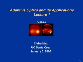
Adaptive Optics and its Applications Lecture 1. Claire Max UC Santa Cruz September 25, 2003. Outline of lecture. Introductions, goals of this course Overview of adaptive optics for astronomy Adaptive optics at UCSC How the course will work Homework for next week.

E N D
Adaptive Optics and its ApplicationsLecture 1 Claire Max UC Santa Cruz September 25, 2003
Outline of lecture • Introductions, goals of this course • Overview of adaptive optics for astronomy • Adaptive optics at UCSC • How the course will work • Homework for next week Please remind me to stop for a break at 2:45 pm: ice cream sundaes downstairs!
Goals of this course • To understand the main concepts behind adaptive optics systems • To understand how to do astronomical observations with AO • Planning, reducing, and interpreting data (your own data, but perhaps more importantly other people’s data) • Some of this will apply to AO for vision science as well • Opportunity to delve into engineering details if you are interested • Brief introduction non-astronomical applications of AO • I hope to interest a few of you in learning more AO, perhaps doing research
Why is adaptive optics needed? Turbulence in earth’s atmosphere makes stars twinkle More importantly, turbulence spreads out light; makes it a blob rather than a point Even the largest ground-based astronomical telescopes have no better resolution than an 8" telescope!
Images of a bright star, Arcturus Speckles (each is at diffraction limit of telescope) Lick Observatory, 1 m telescope ~ 1 arc sec ~ l / D Long exposure image Short exposure image Image with adaptive optics
Turbulence changes rapidly with time Image is spread out into speckles Centroid jumps around (image motion) “Speckle images”: sequence of short snapshots of a star, taken at Lick Observatory using the IRCAL infra-red camera
Turbulence arises in several places tropopause 10-12 km wind flow over dome boundary layer ~ 1 km Heat sources w/in dome stratosphere
Vertical profile of turbulence Measured from a balloon rising through various atmospheric layers
Optical consequences of turbulence blur • Temperature fluctuations in small patches of air cause changes in index of refraction (like many little lenses) • Light rays are refracted many times (by small amounts) • When they reach telescope they are no longer parallel • Hence rays can’t be focused to a point: Point focus Light rays affected by turbulence Parallel light rays
Imaging through a perfect telescope With no turbulence, FWHM is diffraction limit of telescope, ~l / D Example: l / D = 0.02 arc sec for l = 1 mm, D = 10 m With turbulence, image size gets much larger (typically 0.5 - 2 arc sec) FWHM ~l/D 1.22 l/D in units of l/D Point Spread Function (PSF): intensity profile from point source
Characterize turbulence strength by quantity r0 Wavefront of light r0 “Fried’s parameter” • “Coherence Length” r0 : distance over which optical phase distortion has mean square value of 1 rad2 (r0 ~ 15 - 30 cm at good observing sites) • Easy to remember: r0 = 10cm FWHM = 1” at l = 0.5m Primary mirror of telescope
Effect of turbulence on image size • If telescope diameter D >> r0 , image size of a point source is (l / r0) >> (l / D) • r0 is diameter of the circular pupil for which the diffraction limited image and the seeing limited image have the same angular resolution. • r0 10 inches at a good site. So any telescope larger than this has no better spatial resolution! l / D “seeing disk” l / r0
How does adaptive optics help?(cartoon approximation) Measure details of blurring from “guide star” near the object you want to observe Calculate (on a computer) the shape to apply to deformable mirror to correct blurring Light from both guide star and astronomical object is reflected from deformable mirror; distortions are removed
Infra-red images of a star, from Lick Observatory adaptive optics system With adaptive optics No adaptive optics Note: “colors” (blue, red, yellow, white) indicate increasing intensity
When AO system performs well, more energy in core When AO system is stressed (poor seeing), halo contains larger fraction of energy (diameter ~ r0) Ratio between core and halo varies during night AO produces point spread functions with a “core” and “halo” Definition of “Strehl”: Ratio of peak intensity to that of “perfect” optical system Intensity x
Adaptive optics increases peak intensity of a point source Lick Observatory No AO With AO Intensity With AO No AO
Schematic of adaptive optics system Feedback loop: next cycle corrects the (small) errors of the last cycle
How to measure turbulent distortions (one method among many) Shack-Hartmann wavefront sensor
Shack-Hartmann wavefront sensor measures local “tilt” of wavefront • Divide pupil into subapertures of size ~ r0 • Number of subapertures (D / r0)2 • Lenslet in each subaperture focuses incoming light to a spot on the wavefront sensor’s CCD • Deviation of spot position from a perfectly square grid measures shape of incoming wavefront • Wavefront reconstructor computer uses positions of spots to calculate voltages to send to deformable mirror
How a deformable mirror works (idealization) BEFORE AFTER Deformable Mirror Incoming Wave with Aberration Corrected Wavefront
Real deformable mirrors have continuous surfaces • In practice, a small deformable mirror with a thin bendable face sheet is used • Placed after the main telescope mirror
Most deformable mirrors today have thin glass face-sheets Glass face-sheet Light Cables leading to mirror’s power supply (where voltage is applied) PZT or PMN actuators: get longer and shorter as voltage is changed Anti-reflection coating
Deformable mirrors come in many sizes • Range from 13 to > 900 actuators (degrees of freedom) About 12” A couple of inches Xinetics
New developments: tiny deformable mirrors • Potential for less cost per degree of freedom • Liquid crystal devices • Voltage applied to back of each pixel changes index of refraction locally • MEMS devices (micro-electro-mechanical systems)
If there’s no close-by “real” star, create one with a laser • Use a laser beam to create artificial “star” at altitude of 100 km in atmosphere
Laser is operating at Lick Observatory, being commissioned at Keck Keck Observatory Lick Observatory
Laser guide star at Lick Observatory is working well Uncorrected image of a star Laser Guide Star correction Images of a 15th magnitude star, l = 2.2 microns
Astronomical observatories with AO on 3-5 m telescopes • ESO 3.6 m telescope, Chile • University of Hawaii • Canada France Hawaii • Mt. Wilson, CA • Lick Observatory, CA • Mt. Palomar, CA • Calar Alto, Spain } “Curvature sensing” systems > 210 journal articles on AO astronomy, to date
Adaptive optics system is usually behind main telescope mirror • Example: AO system at Lick Observatory’s 3 m telescope Support for main telescope mirror Adaptive optics package below main mirror
Lick adaptive optics system at 3m Shane Telescope DM Off-axis parabola mirror IRCAL infra-red camera Wavefront sensor
Canada France Hawaii Telescope Fifteen minute integration time 0.19 arc sec resolution
Palomar adaptive optics system AO system is in Cassegrain cage 200” Hale telescope
Adaptive optics makes it possible to find faint companions around bright stars Two images from Palomar of a brown dwarf companion to GL 105 200” telescope Credit: David Golimowski
The new generation: adaptive optics on 8-10 m telescopes Summit of Mauna Kea volcano in Hawaii: Subaru 2 Kecks Gemini North And at other places: MMT, VLT, LBT, Gemini South
The Keck Telescope Adaptive optics lives here
Keck Telescope’s primary mirror consists of 36 hexagonal segments Person! Nasmyth platform
Keck AO system performance on bright stars is spectacular! A 9th magnitude star Imaged H band (1.6 mm) Without AO FWHM 0.34 arc sec Strehl = 0.6% With AO FWHM 0.039 arc sec Strehl = 34%
Neptune in infra-red light (1.65 microns) With Keck adaptive optics Without adaptive optics 2.3 arc sec May 24, 1999 June 27, 1999
Details of Neptune’s bright storm at a scale of 400 - 500 km Square root color map Linear color map Each pixel is 0.017 arc sec Dx = 375 km at Neptune H band (1.65 microns)
How to relate IR and visible features? Circumferential bands Compact southern features Visible: Voyager 2 fly-by, 1989 2 mm: Keck adaptive optics, 2000 Compact features such as Great Dark Spot, smaller southern features: probably stable vortices
Near-IR AO image of a volcano erupting on Jupiter’s moon Io Gas plume from a volcanic eruption Credit: Scott Acton Visible-light image from Galileo spacecraft at Io (every dark spot is a volcano) Near-IR image from Keck adaptive optics
Io volcanoes in infrared light Credit: Franck Marchis and Team Keck
VLT NAOS AO first light Cluster NGC 3603: IR AO on 8m ground-based telescope achieves same resolution as HST at 1/3 the wavelength NAOS AO on VLT = 2.3 microns Hubble Space Telescope WFPC2, = 800 nm
Some frontiers of adaptive optics • Current systems (natural and laser guide stars): • How can we monitor the PSF while we observe? • How accurate can we make our photometry be? • What methods will allow us to do high-precision spectroscopy with AO? • Future systems: • Can we push new AO systems to achieve very high contrast ratios, to detect planets around nearby stars? • How can we do AO with laser guide stars on 30-m telescopes of the future?