Download
1 / 77
810 likes | 993 Vues
STM as a Tool to Understand the Electronic Properties of Molecules. Peter Grutter Physics Department McGill University Part of SPM lecture series in 534A ‘Nanoscience and Nanotechnology’. Outline. Motivation and Intro History of tunneling STM and STS theory Wires Molecules

E N D
STM as a Tool to Understand the Electronic Properties of Molecules Peter Grutter Physics Department McGill University Part of SPM lecture series in 534A ‘Nanoscience and Nanotechnology’
Outline • Motivation and Intro • History of tunneling • STM and STS theory • Wires • Molecules • Chemically and atomically defined contacts
First STM Binnig and Rohrer obtained the Nobel prize in 1986 for the discovery of the STM
But: 1972! Topografiner System very similar to today’s STM, but atomic resolution was not achieved 30 A vertical, 4000 A lateral resolution
How does it work? • Tunneling current between tip and sample I ~ (V/s) exp (- A√φ*s)
Tunneling current • Exponential dependence on distance I ~ (V/s) exp (- Aφ1/2s) “Proof of concept” March 18th, 1981 Binnig et al, APL 1982 Very sensitive to gap size!
First STM image • Binnig et al. 1982, PRL • First atomic resolution image of the Si (111) 7x7 reconstruction
Tip preparation • Tip must be as sharp and narrow as possible Chemically etched or mechanically cut.
Tip effects • The shape of the tip may affect the image • More than one tip • “flat” or irregular shape • Structure change during scan
Scan resolution STM Large Range Comparable (or better) to most techniques
Operation of an STM1,2 [1] C. Julian Chen, Introduction to Scanning Tunnelling Microscopy, Oxford (1993) [2] G.A.D. Briggs and A. J. Fisher, Surf. Sci. Rep.33, 1 (1999)
Current theoretical models Theoretical methods: Landauer formula or Keldysh non-equilibrium Green’s functions 1-4 Transfer Hamiltonian methods5 Methods based on the properties of the sample surface alone6 [1] R. Landauer, Philos. Mag. 21, 863 (1970) M. Buettiker et. al. Phys. Rev. B31, 6207 (1985) [2] L. V. Keldysh, Zh. Eksp. Theor. Fiz. 47, 1515 (1964) [3] C. Caroli et al. J. Phys. C4, 916 (1971) [4] T. E. Feuchtwang, Phys. Rev. B10, 4121 (1974) [5] J. Bardeen, Phys. Rev. Lett.6, 57 (1961) [6] J. Tersoff and D. R. Hamann, Phys. Rev. B31, 805 (1985)
[1] Y. Meir and N. S. Wingreen, Phys. Rev. Lett. 68, 2512 (1992) [2] A.A. Abrikosov, L.P. Gorkov and I.E. Dzyaloshinski, Methods of Quantum Field Theory in Statistical Physics, Dover, NY (1975) [3] M. Buettiker et al. Phys. Rev. B31, 6207 (1985) Landauer formula for the STM1,2 The tunnel current for non-interacting electrons3:
[1] J. Pendry et al. J. Phys. Condens Matter3, 4313 (1991) [2] J. Julian Chen, Introduction to Scanning Tunneling Microscopy Oxford (1993) pp. 65 - 69 Transfer Hamiltonian method1,2 M…overlap of wavefunctions (--> resolution!) r…. DOS ( --> spectroscopy !)
[1] C.J. Chen, Introduction to Scanning Tunneling Microscopy, Oxford Univ. Press (1993) [2] W.A. Hofer and J. Redinger, Surf. Sci. 447, 51 (2000) Bardeen approach1,2
Tunneling Current Q…. Workfunction, typically 3-5 eV z….. Tip-sample separation, typically 4-10 A D z = 1 A --> D I one order of magnitude !
Small V approximation! Simmon’s equation (Simmon, 1963) Fowler-Nordheim regime (V>> q) Resolution due to exp dependence! (not so on metals -> later) Measure log I vs log V -> resonances!
Unknown/Challenges: 1. Chemical nature of STM tip (problem for spectroscopy, corrugation) 2. Relaxation of tip/surface atoms (tip sample separation not equal to piezo scale) 3. Effect of tip potential on electronic surface structure (quenching of surface states) 4. Influence of magnetic properties on tunnelling current/surface corrugation (is spin-STM possible?) 5. Relative importance of the effects
[1] P. Varga and M. Schmid, Appl. Surf. Sci. 141, 287 (1999) 1. Chemical nature of the tip1
[1] G. Kresse and J. Hafner, Phys. Rev. B47, R558 (1993) [2] Ph. Kurz et al.J. Appl. Phys.87, 6101 (2000) [3] J. P. Perdew et al. Phys. Rev. B46, 6671 (1992) Model of the STM tip1,2,3 Number of layers: 7 Free standing film Numerical method: DFT Relaxations: VASP [1] Electronic structure: FLEUR [2] Lattice constant: 6.016 au (GGA) Exchange/correlation: PW91[3] Brillouin-zone sampling: 10 k-points Convergence parameter: < 0.01 e/au3
[1] P.T. Wouda et al. Surf. Sci. 359, 17 (1996) [2] P. Varga and M. Schmid Appl. Surf. Sci. 141, 287 (1999) Chemical contrast on PtRh(100)1,2 Experiments: 22 pm contrast Simulations: interval EF +/- 80 meV
[1] W.A. Hofer, A.J. Fisher, R.A. Wolkow, and P. Grutter, Phys. Rev. Lett 87, 236104 (2001) [2] G. Cross, A. Schirmeisen, P. Grutter, U. Durig, Phys. Rev. Lett. 80, 4685 (1998) 2. The influence of forces in STM scans1 Force measurement on Au(111)2 Simulation of forces: Simulation: VASP GGA: PW91 4x4x1 k-points
Tip relaxation effects The force on the apex atom is one order of magnitude higher than forces in the second layer W tip on Au(111) surface Substantial Relaxations occur only in a distance range below 5A
Tip relaxation effects Hofer, Fisher, Wolkow and Grutter Phys. Rev. Lett. 87, 236104 (2001) W tip on Au(111) surface The real distance is at variance with the piezoscale by as much as 2A The surplus current due to relaxations is about 100% per A
[1] V. M. Hallmark et al., Phys. Rev. Lett. 59, 2879 (1987) Corrugation enhancement STM simulation: bSCAN Bias voltage: - 100mV Energy interval: +/- 100meV Current contour: 5.1 nA Due to relaxation effects in the low distance regime the corrugation of the Au(111) surface is enhanced by about 10-15 pm1
[1] W.A. Hofer, J. Redinger, A. Biedermann, and P. Varga, Surf. Sci. Lett.466, L795 (2000) [2] V. L. Moruzzi et al. Phys. Rev. B15, 6671 (1977) 3. Change of electronic surface properties1 System: Fe(100) bcc lattice DFT calculation: FLEUR Lattice constant: 2.78 A LDA: Moruzzi et al [2] No of k-points: 36
Quenching of surface states Simulation of quenching: distance dependent reduction of the occupation number of single Kohn-Sham states of the surface, 2nd order polynomial
Elastic: linear I-V Inelastic: non-linear I-V Tunneling Spectroscopy (cartoon version)
Tunneling Spectroscopies • I(V) at constant z or variable z • dI/dV at constant z or constant average I • d (log I)/dz (barrier height measurement)
Tunneling Spectroscopy: an example Hyrogen on SiC surface: goes from insulator -> conductor Derycke et al., Nature Mater. 2, 253 (2003) UPS
Geometric and Electronic Properties of Molecules I Alkane thiols Porphrin on Au(111) P. Weiss et al., Science 271, 1705 (1996) Y. Sun, H. Mortensen, F. Mathieu, P. Grutter (McGill)
Geometric and Electronic Properties of Molecules II C60 on Au(111) J. Mativietsky, S. Burke, Y.Sun, S. Fostner, R. Hoffmann, P. Grutter
Single-Molecule Vibrational Spectroscopy and Microscopy 25 averages, 2 minutes per spectrum Ds/s= 4.2% (1-2) Ds/s= 3.3% (3, different molecule) B.C. Stipe, M.A. Rezaei, W. Ho Science 280, 1733 (1998)
C2H2 and C2D2 comparison Single-Molecule Vibrational Spectroscopy and Microscopy B.C. Stipe, M.A. Rezaei, W. Ho Science 280, 1733 (1998)
Geometric and Electronic Properties of Nanowires I 0.3 ML Cs on GaAs and InSb (fig. C) Whitman et al, PRL 66, 1338 (1991)
Geometric and Electronic Properties of Nanowires II 0.36 ML Ho on Si, 400 nm image Anisotropic lattice mismatch --> wires. Are they conductive? Ohbuchi and Nogami, PRB 66, 165323 (2003)
Geometric and Electronic Properties of Nanowires III 0.04 ML In on Si(001), 14 nm image However: In wires are NOT conductive ! Nogami, Surf. Rev. & Letters, 6, 1067 (1999) Evans and Nogami, PRB 59, 7644 (1999)
Defined, reproducible, understandable I-V of molecules Chemically reliable contact Cui et al. Nanotechnology 13, 5 (2002), Science 294, 571 (2001)
Other spectroscopies of molecules: may the force be with you Experimental variation o f the conductance of C60 modulated by Vin (t). The time variation o f the voltage Vz piezo applied to the piezoelectric actuator is shown as a dashed line and the experimental C60(t) conductance response as a solid line. Ch. Joachim and J. Gimzewski, Chem. Phys. Lett 265, 353 (1997)
Interpretation of C60 amplifier Calculated variations of surface resistance of C60 on Au(110) as a function of applied force Ch. Joachim and J. Gimzewski, Proc. IEEE 86, 184 (1998)
STM/STS and conductivity So if STM/STS is so powerful - can we use it to determine the conductivity of molecules???
Calculating Conductance ‘Traditional’: infinite, structureless leads -> periodic boundary conditions. but: - result depends on lead size! - bias not possible due to periodic boundary condition! Jellium lead Jellium lead molecule
lead ab-initio modelling of electronic transport Hong Guo’s research group, McGill Physics
DFT plus non-equilibrium Green’s Functions J. Taylor, H. Guo , J. Wang, PRB 63, R121104 (2001) 1. Calculate long, perfect lead. Apply external potential V by shifting energy levels -> create electrode data base and get potential right lead
2. Solve Poisson equation for middle part (device plus a bit of leads); match wavefunctions and potential as a function of V to leads (use data base) in real space. 3. calculated with non-equilibrium Green’s functions (necessary as this is an open system). This automatically takes care of bound states