Download
1 / 62
630 likes | 802 Vues
Lecture L03 AST3021 Celestial Mechanics 1. Precession of orbits and rotational axes Perturbation theory of orbits: 2.General (analytical) - relativistic precession, solar sail 3. Special (numerical) - Euler and RK methods of integration 4. Integrals of motion method

E N D
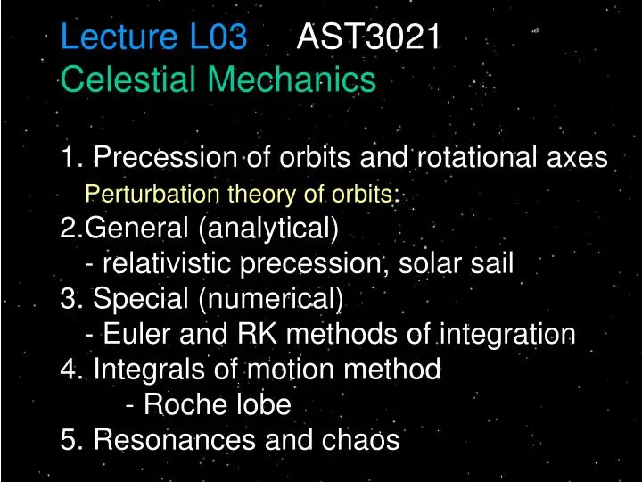
Lecture L03 AST3021 Celestial Mechanics 1. Precession of orbits and rotational axesPerturbation theory of orbits: 2.General (analytical) - relativistic precession, solar sail 3. Special (numerical) - Euler and RK methods of integration 4. Integrals of motion method - Roche lobe 5. Resonances and chaos
Precession orbit precession, spin axis precession Praecedere [latin] = to precede 4 3 7 1 2 6 2 3 5 4 1 Exceptions (closed orbits): two force laws only: F~1/r^2, F~r (Bertrand’s theorem)
Angular momentum vector shifted sideways by torque, value preserved ==> precession. dL =( torque ) dt dL =( r x F ) dt r x F r dL F
Torque on satellite’s orbit = -N Torque on the planet = N Velocity of precession = N ==> angular speed can be computed L3 satellite planet Satellite, 1/2 P later
Obliquity (inclination) perturber mass r = perturber distance Earth axis’ precession (angular speed): I1,2,3 = three moments of inertia of the Earth, satisfying: (from Earth flattenig) L3 The corresponding period of precession of Earth axis = 33000 yr (from the Moon), and 81000 (from the sun) Combined luni-solar precession has period 26000 yr = 51”/yr (Note: 1/33000 + 1/81000 = 1/26000, angular speeds, not periods, add up). This affects right ascention of objects in catalogues and maps, which therefore must state the “epoch” of coordinates.
General theory of perturbations (analytical) Joseph-Louis Lagrange (1736-1823)
1st order perturbation theories philosophy: perturbation (variables with index 1) are evaluated along the unperturbed trajectory (index 0) expanded as 1st order perturbation equations Carl F. Gauss used the radial (R) and transversal (T) components of perturbing forces (accelerations) to compute torque (r T) and the orbital energy drain/gain rate (dE/dt = force * dr/dt) to find along the unperturbed orbit
ellipse n = ‘mean motion’ = mean angular speed, often designated by in other contexts (R, T) = time-dependent components of perturbing force (acceleration)
(Derived like da/dt, from energy and angular momentum change) change variables and use the equation of ellipse for r(θ): r = a(1-e^2) /(1+ e cos (θ))
The relativistic precession of orbits as one of the applications of general perturbation theory (we’ll cheat a little by using Newtonian dynamics with a modified potential, approximating the use of general relativity; that kind of cheating is quite OK!). (1879-1955) (drawing not to scale, shape and the precession exaggerated!)
true anomaly (orbital angle) longitude of periastron We will use solar sail problem to illustrate three different approaches to celestial mechanics: two perturbation theories and the energy method toward the sun to the sun
e(t) = sin (t/te), where te = (2na)/(3f), until e=1 after time (pi/2)te. During this evolution, orbit is elongated perpendicular to the force! f
Special theory of perturbations (numerical) Most popular numerical integration methods for ODEs Euler method (1st order) & Runge-Kutta (2nd - 8th order) Leonard Euler Carle Runge Martin Kutta 1856-1927 1867-1944
The Euler method • We want to approximate the solution of the differential equation • For instance, the Kepler problem which is a 2nd-order equation, can be • turned into the 1st order equations by introducing double the number of • equations and variables: e.g., instead of handling the second derivative • of variable x, as in the Newton’s equations of motion, one can integrate the • first-order (=first derivative only) equations using variables x and vx = dx/dt • (that latter definition becomes an additional equation to be integrated). • Starting with the differential equation (1), we replace the derivative • y' by the finite difference approximation, which yields the following formula • which yields • This formula is usually applied in the following way.
The Euler method (cont’d) • This formula is usually applied in the following way. • We choose a step size h, and we construct the sequence t0, • t1 = t0 + h, t2 = t0 + 2h, ... We denote by yn a numerical estimate of • the exact solution y(tn). Motivated by (3), we compute these estimates • by the following recursive scheme • yn + 1 = yn + h f(tn,yn). • This is the Euler method (1768), probably • invented but not formalized earlier by Robert Hook. • It’s a first (or second) order method, meaning that • the total error is ~h 1 (2) It requires small time steps • & has only moderate accuracy, but it’s very simple!
The classical fourth-order Runge-Kutta method • One member of the family of Runge-Kutta methods is so commonly used, • that it is often referred to as "RK4" or simply as "the Runge-Kutta method". • The RK4 method for the problem • is given by the following equation: • where • Thus, the next value (yn+1) is determined by the present value (yn) plus the • product of the size of the interval (h) and an estimated slope.
Runge-Kutta 4th order (cont’d) • Thus, the next value (yn+1) is determined by the present value (yn) plus the • product of the size of the interval (h) and an estimated slope. The slope is • a weighted average of slopes: • k1 is the slope at the beginning of the interval; • k2 is the slope at the midpoint of the interval, using slope k1 to determine the value of y at the point tn + h/2 using Euler's method; • k3 is again the slope at the midpoint, but now using the slope k2 to determine the y-value; • k4 is the slope at the end of the interval, with its y-value determined using k3. • When the four slopes are averaged, more weight is given to the midpoint. • The RK4 method is a fourth-order method, meaning that the total error is ~h4. It allows larger time steps & better accuracy than low-order methods. Thus, the next value (yn+1) is determined by the present value (yn) plus the product of the size of the interval (h) and an estimated slope
Solar sail problem revisited: A y/a A C A B C B f x/a Numerical integration (Euler method, h=dt=0.001 P) Comparing the numerical results with analytical perturbation theory we see a good agreement in case A of small perturbations, f << 1. In this limit, analytical results are more elegant and general (valid for every f) than numerical integration: For instance, e(t) = sin (t/te), where te = (2na)/(3f), for all sets of f, n, a. x
Solar sail problem revisited: B, C y/a A C A B C B f x/a Numerical integration (Euler method, h=dt=0.001 P) For instance, e(t) = sin (t/te), where te = (2na)/(3f), for all f, n, a. x However, in cases B and C of large perturbations, f ~ 0.1…1. In this limit, analytical treatment cannot be used, because the assumptions of the theory are not satisfied (changes of orbit are not gradual). Eccentricity becomes undefined after a fraction of the orbit (case B, C). In this case, the computer is your best friend, though it requires a repeated calculation for each f, and introduces numerical error.
INTEGRALS OF MOTION 1. Energy methods (integrals of motion) 2. Zero Vel. Surfaces (Curves) and the concept of Roche lobe 3. Roche lobe radius calculation 4. Lagrange points and their stability 5. Hill problem and Hill stability of orbits 6. Resonances and stability of the Solar System
Non-perturbative methods (energy constraints, integrals of motion) Karl Gustav Jacob Jacobi (1804-1851)
Solar sail problem again A standard trick to obtain energy integral
Energy criterion guarantees that a particle cannot cross the Zero Velocity Curve (or surface), and therefore is stable in the Jacobi sense (energetically). However, remember that this is particular definition of stability which allows the particle to physically collide with the massive body or bodies -- only the escape from the allowed region is forbidden! In our case, substituting v=0 into Jacobi constant, we obtain:
Allowed regions of motion in solar wind (hatched) lie within the Zero Velocity Curve f=0 f=0.051 < (1/16) particle cannot escape from the planet located at (0,0) f=0.063 > (1/16) f=0.125 particle can (but doesn’t always do!) escape from the planet (cf. numerical cases B and C, where f=0.134, and 0.2, much above the limit of f=1/16).
Circular Restricted 3-Body Problem (R3B) L4 L1 L3 L2 Joseph-Louis Lagrange (1736-1813) [born: Giuseppe Lodovico Lagrangia] L5 “Restricted” because the gravity of particle moving around the two massive bodies is neglected (so it’s a 2-Body problem plus 1 massless particle, not shown in the figure.) Furthermore, a circular motion of two massive bodies is assumed. General 3-body problem has no known closed-form (analytical) solution.
NOTES: The derivation of energy (Jacobi) integral in R3B does not differ significantly from the analogous derivation of energy conservation law in the inertial frame, e.g., we also form the dot product of the equations of motion with velocity and convert the l.h.s. to full time derivative of specific kinetic energy. On the r.h.s., however, we now have two additional accelerations (Coriolis and centrifugal terms) due to frame rotation (non-inertial, accelerated frame). However, the dot product of velocity and the Coriolis term, itself a vector perpendicular to velocity, vanishes. The centrifugal term can be written as a gradient of a ‘centrifugal potential’ -(1/2)n^2 r^2, which added to the usual sum of -1/r gravitational potentials of two bodies, forms an effective potential Phi_eff. Notice that, for historical reasons, the effective R3B potential is defined as positive, that is, Phi_eff is the sum of two +1/r terms and +(n^2/2)r^2
Effective potential in R3B mass ratio = 0.2 The effective potential of R3B is defined as negative of the usual Jacobi energy integral. The gravitational potential wells around the two bodies thus appear as chimneys.
Lagrange points L1…L5 are equilibrium points in the circular R3B problem, which is formulated in the frame corotating with the binary system. Acceleration and velocity both equal 0 there. They are found at zero-gradient points of the effective potential of R3B. Two of them are triangular points (extrema of potential). Three co-linear Lagrange points are saddle points of potential.
Jacobi integral and the topology of Zero Velocity Curves in R3B rL = Roche lobe radius + Lagrange points
Sequence of allowed regions of motion (hatched) for particles starting with different C values (essentially, Jacobi constant ~ energy in corotating frame) High C (e.g., particle starts close to one of the massive bodies) Highest C Low C (for instance, due to high init. velocity) Notice a curious fact: regions near L4 & L5 are forbidden. These are potential maxima (taking a physical, negative gravity potential sign) Medium C
= 0.1 C = R3B Jacobi constant with v=0 Édouard Roche (1820–1883), Roche lobes terminology: Roche lobe ~ Hill sphere ~ sphere of influence (not really a sphere)
Is the motion around Lagrange points stable? Stability of motion near L-points can be studied in the 1st order perturbation theory (with unperturbed motion being state of rest at equilibrium point).
Stability of Lagrange points Although the L1, L2, and L3points are nominally unstable, it turns out that it is possible to find stable and nearly-stable periodic orbits around these points in the R3B problem. They are used in the Sun-Earth and Earth-Moon systems for space missions parked in the vicinity of these L-points. By contrast, despite being the maxima of effective potential, L4 and L5 are stable equilibria, provided M1/M2 is > 24.96 (as in Sun-Earth, Sun-Jupiter, and Earth-Moon cases). When a body at these points is perturbed, it moves away from the point, but the Coriolis force then bends the trajectory into a stable orbit around the point.
Observational proof of the stability of triangular equilibrium points Greeks, L4 Trojans, L5 From: Solar System Dynamics, C.D. Murray and S.F.Dermott, CUP
Roche lobe radius depends weakly on R3B mass parameter = 0.1 = 0.01
Computation of Roche lobe radius from R3B equations of motion ( , a = semi-major axis of the binary) L
Roche lobe radius depends weakly on R3B mass parameter m2/M = 0.01 (Earth ~Moon) r_L = 0.15 a m2/M = 0.003 (Sun- 3xJupiter) r_L = 0.10 a m2/M = 0.001 (Sun-Jupiter) r_L = 0.07 a m2/M = 0.000003 (Sun-Earth) r_L = 0.01 a = 0.1 = 0.01
Hill problem George W. Hill (1838-1914) - studied the small mass ratio limit of in the R3B, now called the Hill problem. He ‘straightened’ the azimuthal coordinate by replacing it with a local Cartesian coordinate y, and replaced r with x. L1 and L2 points became equidistant from the planet. Other L points actually disappeared, but that’s natural since they are not local (Hill’s equations are simpler than R3B ones, but are good approximations to R3B only locally!) Roche lobe ~ Hill sphere ~ sphere of influence(not really a sphere, though)