Download

1 / 31
320 likes | 378 Vues
Explore data compression techniques including Huffman coding and arithmetic coding in this informative text. Learn about entropy, modeling strategies, coding methods, and more. Discover how to efficiently encode information for optimal compression results.

E N D
Pasi Fränti Information theoryData compression perspective 4.2.2016
Bits and Codes One bit: 0 and 1 Two bits: 00, 01, 10, 11 Four bits: 0000, 0001, 0010 … 1111 (8 values) Eight bits: 2256 values (e.g. ASCII code) k bits 2k values N values log2N bits
Entropy Self-entropy of symbol Entropy of source
Prefix code Example of a prefix code a = 0 b = 10 c = 110 d = 111 Example of non-prefix code a = 0 b = 01 c = 011 d = 111 4
Huffman coding Codetree Symbols and frequencies First step of the process 7
Two coding methods • Huffman coding • David Huffman, 1952 • Prefix code • Bottom-up algorithm for construction of the code tree • Optimal when probabilities are of the form 2n • Arithmetic coding • Rissanen, 1976 • General: applies to any source • Suitable for dynamic models (no explicit code table) • Optimal for any probability model • All input file is coded as one code word 9
Work space 10
Static or adaptive model Static: + No side information + One pass over the data is enough - Fails if the model is incorrect Semi-adaptive: + Optimizes model to the input data - Two-passes over the image needed - Model must also be stored in the file Adaptive: + Optimizes model to the input data + One pass over the data is enough - Must have time to adapt to the data 12
Using wrong model ESTIMATED MODEL: CORRECT MODEL: AVERAGE CODE LENGTH: INEFFICIENCY: 13
Summary of context model NO CONTEXT: fw = 56, fb = 8, pw = 87.5 %, pb = 12.5 % Total bit rate = 10.79 + 24 = 34.79 Entropy = 34.79 / 64 = 0.54 bpp PIXEL ABOVE: Total bit rate = 33.28 Entropy = 33.28 / 64 = 0.52 bpp PIXEL TO LEFT: Total bit rate = 7.32 Entropy = 7.32 / 64 = 0.11 bpp 16
Block coding • Two problems: • Impossible to make code table for binary input • Cannot use fractions of bits (p=0.9 H=0.07 bits) • Solution 1: Block coding • Block symbols • Contradicts context model • Alphabet explode exponentially with the number of symbols: • 3-symbol blocks 2563=16 M • Solution 2: Arithmetic coding • Block entire input! • No explicit code table
Arithmetic coding principles • Length of interval = A • Coding of A takes –log2A bits • Divides the interval according to the probabilities • The lengths of the subintervals sums up to 1. 1 1 c 0.9 b 0.75 0.7 a 0.50 Probabilities: p(a) = 0.7 p(b) = 0.2 p(c) = 0.1 0.25 0 0 25
Coding examplesequence aab Probabilities: p(a) = 0.7 p(b) = 0.2 p(c) = 0.1 A = 0.098 H = -log 0.098 = 3.35 bits 26
Coding of sequence aab Probabilities: 1 1 1 p(a) = 0.7 p(b) = 0.2 p(c) = 0.1 c 0.9 b 0.75 0.75 0.7 0.70 c a 0.63 b 0.49 0.50 0.50 0.490 a c 0.441 b b 0.343 a 0.25 0.25 0 0 0 0 0 27
Code length Length of the final interval: It’s code length: Length with respect to the distribution: 28
Optimality of Arithmetic Coding • Interval is not exactly power of 2. • Round it down to A’ < A that is power of 2 Lower bound for interval size: Upper bound for code length: Length with respect to the distribution: 29
/* Initialize lower and upper bounds */ low 0; high 1; cum[0] 0; cum[1] p1; /* Calculate cumulative frequencies */ FOR i 2 TO k DO cum[i] cum[i-1] + pk WHILE Symbols left> DO /* Select the interval for symbol c */ c READ(Input); range high - low; high low + range*cum[c+1]; low low + range*cum[c]; /* Initialize lower and upper bounds */ low 0; high 1; cum[0] 0; cum[1] p1; /* Calculate cumulative frequencies */ FOR i 2 TO k DO cum[i] cum[i-1] + pk WHILE Symbols left> DO /* Select the interval for symbol c */ c READ(Input); range high - low; high low + range*cum[c+1]; low low + range*cum[c]; /* Half-point zooming: lower */ WHILE high < 0.5 DO high 2*high; low 2*low; WRITE(0); FOR buffer TIMES DO WRITE(1); buffer 0; /* Half-point zooming: higher */ WHILE low > 0.5 DO high 2*(high-0.5); low 2*(low-0.5); WRITE(1); FOR buffer TIMES DO WRITE(0); buffer 0; /* Quarter-point zooming */ WHILE (low > 0.25) AND (high < 0.75) THEN high 2*(high-0.25); low 2*(low-0.25); buffer buffer + 1;
Working space Text box 0.75