Download

1 / 15
150 likes | 319 Vues
Modeling Price Elasticity. Kiran Ravulapati, Katia Frank, Wassim Chaar Delta Technology, Atlanta, GA 30354. What is Price Elasticity ?. Price Elasticity (PE) A PE of -1.5 means there is a 1.5% drop in demand for a 1% increase in price. Price Elasticity - Literature.

E N D
Modeling Price Elasticity Kiran Ravulapati, Katia Frank, Wassim Chaar Delta Technology, Atlanta, GA 30354
What is Price Elasticity ? • Price Elasticity (PE) • A PE of -1.5 means there is a 1.5% drop in demand for a 1% increase in price.
Price Elasticity - Literature • Past research modeled price elasticity at a macro level using aggregated, high level data. - Oum, Tae H., Zhang, Anmin and Zhang, Yimin (1993) “Inter-Firm Rivalry and Firm-Specific Price elasticities in Deregulated Airline Markets,” Journal of Transport Economics and Policy,27, 171-192 • Price elasticity at product level received little attention. Perhaps, this is because of the revenue management effects involved.
Price Elasticity - Assumptions • We modeled simple price elasticity only. Interaction between products is not considered. • We studied the ‘vacuum’ scenario i.e., all airlines in the market have same prices. • Revenue management effects are consistent.
Bookings for market XXX-YYY Discounted Coach demand 0-10 30-40 60-70 90-100 120-130 150-160 180-190 210-220 240-250 270-280 300-310 330-340 360-370 390-400 420-430 fareband Price Elasticity - “Vacuum” Step 1: Divide historical demand/price data into fare bands.
Price Elasticity - “Vacuum” Step 2: Remove RM effect by cumulating demand. Bookings for market XXX-YYY Discounted Coach Cumulative Demand 0-10 30-40 60-70 90-100 120-130 150-160 180-190 210-220 240-250 270-280 300-310 330-340 360-370 390-400 420-430 fareband
Price Elasticity - “Vacuum” Step 3: Adjust the curve for sell up. Bookings for market XXX-YYY Discounted Coach Cumulative Demand Adjusted Cumulative Demand 0-10 30-40 60-70 90-100 120-130 150-160 180-190 210-220 240-250 270-280 300-310 330-340 360-370 390-400 420-430 fareband
Price Elasticity - Sell Up Total Demand = 16 + 50 + 30 = 96 Demand 20 50 30 $50-$70 $70-$90 $90-$110 0.8*20 = 16 30
Price Elasticity - “Vacuum” Step 4: Fit a function to the adjusted demand curve using regression analysis and calculate price elasticity. Price Vs Demand Curve for market XXX-YYY Discounted Coach Demand 0-10 30-40 60-70 90-100 120-130 150-160 180-190 210-220 240-250 270-280 300-310 330-340 360-370 390-400 420-430 fareband
Price Elasticity - Summary • This model is a first step towards developing a methodology for price elasticity. • Select a representative sample of historical data. • Group only similar markets/products for this analysis. • To capture seasonal changes in prices, this analysis should be repeated for each season using new data.
Price Elasticity - Summary • Revenue management effects, spill and capacity limits, should be used to determine the impact of fare increase/decrease. • Methodology can be used at various aggregate levels - market/region/airline/products. • Possible extensions - Impact of fare rules - Interaction between substitutable products