Download
1 / 60
600 likes | 751 Vues
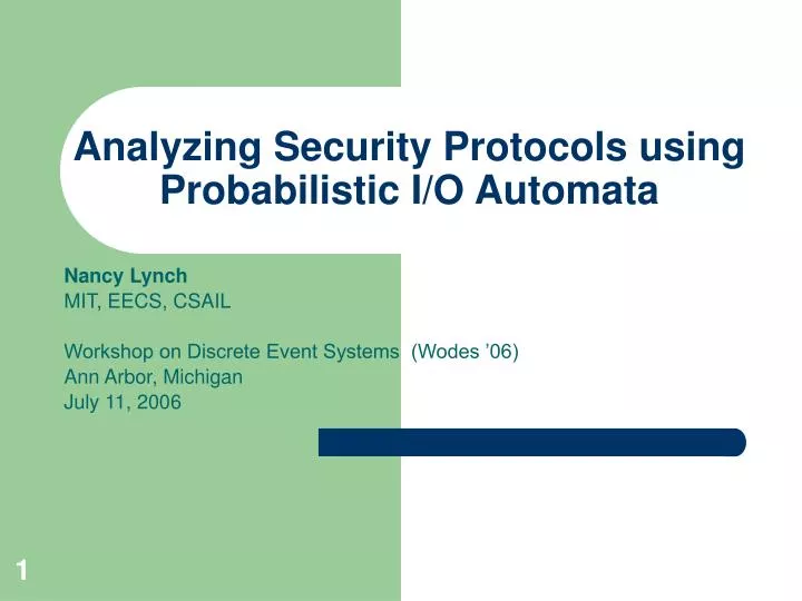
Analyzing Security Protocols using Probabilistic I/O Automata. Nancy Lynch MIT, EECS, CSAIL Workshop on Discrete Event Systems (Wodes ’06) Ann Arbor, Michigan July 11, 2006. Authors: Ran Canetti, Ling Cheung, Dilsun Kaynar, Moses Liskov, Nancy Lynch, Olivier Pereira, Roberto Segala

E N D
Analyzing Security Protocols using Probabilistic I/O Automata Nancy Lynch MIT, EECS, CSAIL Workshop on Discrete Event Systems (Wodes ’06) Ann Arbor, Michigan July 11, 2006
Authors: Ran Canetti, Ling Cheung, Dilsun Kaynar, Moses Liskov, Nancy Lynch, Olivier Pereira, Roberto Segala Using Probabilistic I/O Automata to Analyze an Oblivious Transfer Protocol. MIT CSAIL-TR-2005-1001, August ‘05. Revision, CSAIL-TR-2006-046, June ‘06. Task-Structured Probabilistic I/O Automata. WODES ’06. Full version in progress. Using Task-Structured Probabilistic I/O Automata to Analyze an Oblivious Transfer Protocol. CSAIL-TR-2006-047, June ‘06. Time-Bounded Task-PIOAs: A Framework for Analyzing Security Protocols. DISC ’06. References
General goals • Develop techniques for • Modeling security protocols precisely. • Proving their correctness rigorously. • Techniques should handle both functional correctness and security properties. • Should be able to describe cryptographic primitives, computational limitations. • Tractable, usable methods.
I/O Automata models and methods • Our favorite tools for modeling, analyzing distributed algorithms, communication protocols, safety-critical systems,… • Describe systems using: • I/O Automata (IOA) [Lynch, Tuttle] • Timed I/O Automata (TIOA) [Kaynar, Lynch, Segala, Vaandrager] • Hybrid I/O Automata (HIOA) [Lynch, Segala, Vaandrager] • Probabilistic I/O Automata (PIOA) [Segala, Lynch] • Prove correctness using: • Compositional methods: Infer properties of a system from properties of its pieces. • Invariant assertions: Properties that hold in all reachable system states. • Simulation relations: Relate system descriptions at different levels of abstraction.
Uses of I/O Automata • Basic I/O Automata: • Basic distributed algorithms: Consensus, mutual exclusion, spanning trees,… • Timed I/O Automata: • Communication protocols. • Timing-sensitive distributed algorithms. • Simple hybrid systems. • Hybrid I/O Automata: • More complex hybrid systems (controlled vehicles, aircraft). • Mobile ad hoc networks. • Probabilistic I/O Automata: • Randomized distributed algorithms. • So, they should work for Security Protocols too!
An early attempt [Lynch, CSFW 99] • I/O Automata models and proofs of shared-key communication systems • Models: • Diffie-Hellman key distribution protocol, and • Shared-key communication protocol that uses the keys. • Proves correctness and secrecy for the complete system, using a composition theorem. • No probabilities used here---just plain I/O Automata. • Treats the cryptosystem formally (algebraically) not computationally.
Limitations of this approach • Doesn’t describe some key features of cryptographic protocols: • Computational limitations. • Probabilistic behavior. • Small probabilities of guessing secret information. • “Knowledge” of a fact (rather than a value). • So, we decided we needed a modeling framework that supports these features too.
Adv in(i) in(x0,x1) out(xi) Trans Rec New, concrete goal • Prove correctness of a simple 2-party Oblivious Transfer protocol [Goldreich, Micali, Wigderson 87]. • Oblivious Transfer requirements: • Transmitter gets input bits, x0 and x1, from the “Environment”. • Receiver gets input bit i, an index it uses to choose an input. • Receiver should output only the chosen Transmitter input xi. • Adversary (who hears all communication) shouldn’t learn anything. • Requirements include both functional correctness and secrecy properties.
Four versions of the problem • Depending on whether Transmitter and/or Receiver is corrupted. • Adversary also sees inputs, outputs, random choices of corrupted parties. • But it should not learn anything else.
Adv in(i) in(x0,x1) out(xi) Trans Rec Oblivious Transfer Protocol • Trans chooses a random trap-door permutation f, sends to Rec. • Rec chooses random numbers y0 and y1, computes f(yi), where i is its input, keeps y(1-i) unchanged, sends results to Trans. • Trans applies f-1 to both, extracts hard-core bits, xors them with its inputs x0 and x1, sends results back to Rec. • Rec decodes the chosen value.
in(i) in(x0,x1) Sim out(xi) Funct in(i) in(x0,x1) out(xi) Funct out’(xi) Sim PIOA modeling • Use PIOAs to model both protocol and requirements specification. • E.g. Specification, when no one is corrupted: • Specification, when Rec is corrupted:
Adv Sim in(i) in(x0,x1) out(xi) in(i) Trans Rec in(x0,x1) out(xi) Funct Showing the protocol “implements” the specification system: • Uses new implementation notion, ≤neg,pt. • Relates Protocol PIOA system to Specification PIOA system. • “For every poly-time-bounded environment PIOA E, every probabilistic execution of Protocol + E yields “approximately the same” external behavior as some probabilistic execution of Spec + E.” • Approximation: Negligible difference in probability that E “accepts”. • Expresses functional correctness and secrecy.
Proving correctness • Break the proof into several stages, using system descriptions at several levels of abstraction. • Prove some stages using PIOA simulation relations. • Assertions relating states of the two PIOAs. • Use a new type of simulation relation, more general than previous PIOA simulation relations. • Can express complex correspondences between random choices at different levels. • These prove not just ≤neg,pt , but stronger ≤0. • Other stages involve secrecy aspects of a cryptographic primitive (a trap-door function). • Proofs adapted from computational crypto “Distinguisher” arguments. • Usually proved by contradiction. • We recast in terms of mappings between PIOAs, without contradictions.
What’s new here? • Modeling everything, in complete detail, using PIOAs: • Protocols. • Requirements, including functionality and secrecy. • Proofs using simulation relations, in several stages. • Some stages use PIOA simulation relations. • Other stages express Distinguisher arguments. • Separates different types of reasoning. • Needed some new PIOA theory: • Task-PIOAs, for resolving scheduling nondeterminism. • A new kind of simulation relation. • A way to express polynomial-time computation restrictions. • New ways of expressing computational crypto reasoning: • Redefine cryptographic primitives using ≤neg,pt. • Infer ≤neg,pt for systems that use the primitives.
Related work • [Segala 95] Probabilistic I/O Automata theory • [Canetti 01] Universally Composable (UC) security • [Pfitzmann, Waidner 01], [Backes, Pfitzmann, Waidner 04] Composable security • [Mitchell et al.] Modeling/analyzing security protocols using process algebras, with probabilistic poly-time processes. • [Shoup 04] Cryptography proof sketches using many levels of abstraction (“games”). • Work on protocol proofs using formal cryptography, e.g., [Dolev, Yao 83], [Lynch 99]. • Work on protocol proofs using computational cryptography. • Work relating the two, e.g. [Abadi, Rogaway 02], [Canetti, Herzog 05].
Talk Outline: • Overview (done) • Task-PIOAs • PIOAs (review) • Task-PIOA definitions • New simulation relation • Adding computational limitations • Oblivious Transfer Modeling and Analysis • Specification model • Protocol model • Correctness theorems • Modeling the cryptographic primitives • Correctness proof • Conclusions
2.1. PIOAs [Segala] A PIOA P consists of: Q: a countable set of states, q: a start state, I, O, and H: countable sets of input, output, and internal actions D, a transition relation---a set of triples of the form (state, action, probability measure on states). Axioms: Input-enabling Next-transition determinism PIOAs can make both Nondeterministic choices (next action), and Probabilistic choices (next state). Closed PIOA: No input actions.
PIOAs • Scheduler for a PIOA P: • Chooses the next action (fine-grained control). • Choice may depend on entire prior history (full information). • PIOA + Scheduler yield: • Probabilistic execution • Trace distribution (probability measure on sequences of external actions) • Operations: • Composition • Hiding (of output actions) • Simulation relation notion • Relates states to distributions on states. • Implies inclusion of sets of trace distributions.
PIOAs • Traditional PIOA schedulers are too powerful for the security protocol setting: • Choose the next action (fine-grained control). • Choice may depend on entire prior history (full information). • In particular, scheduling choices may depend on secret information, supposedly hidden in the states of non-corrupted protocol participants. • Scheduler can “leak” secret information to adversarial parties, by encoding it in the choices of scheduled actions. • This led us to define more restricted, partial-information “task schedulers”.
2.2. Task-PIOA definitions • Task-PIOA T = (P,R) • PIOA + equivalence relation on output and internal actions. • Task: Equivalence class • E.g., “send” actions for round 1 messages. • Action determinism: At most 1 action in each task enabled in each state. • Task schedule: Arbitrary sequence of tasks. • Models an oblivious task scheduler. • Does not depend on dynamic information generated during execution. • Applying a task schedule to the initial state: • Resolves all nondeterminism. • Yields unique probabilistic execution, unique trace distribution. • More generally, we can applying a task schedule to: • A probability distribution on states, or even • A probability distribution on finite executions.
Task-PIOA operations • Composition: • Compose the PIOAs. • Take the union of the sets of tasks. • Hiding (of actions).
Task-PIOA implementation relation • Environment E for T: • Task-PIOA that “closes” T. • Has special “accept” output action. • Used to express E’s distinguishing power. • T1 ≤0 T2: • For every environment PIOA E for both T1 and T2, every trace distribution of T1 || E (obtained from any task schedule) is also a trace distribution of T2 || E (obtained from some task schedule).
Task-PIOA Compositionality • Theorem: If T1 ≤0 T2 then T1 || T3 ≤0 T2 || T3. • Proof: Straightforward, because of the way the implementation notion ≤0 is defined (in terms of mappings from environments to sets of trace distributions).
2.3. New kind of simulation relation • For comparable, closed task-PIOAs T1 and T2. • ε1 R ε2, for probability measures ε1 and ε2 on finite execs of T1 and T2 with the same trace distribution. • Uses expansion operator Exp(R) on such relations R. • Two conditions (slightly simplified): • Start condition: Start states of T1 and T2 are R-related. • Step condition: There is a mapping c from tasks of T1 to finite sequences of tasks of T2 such that, if ε1 R ε2 and t is a task of T1, then apply(ε1,t) Exp(R) apply(ε2,c(t)). • More general than requiring apply(ε1,t) R apply(ε2,c(t)). • Soundness: Every trace distribution of T1 is a trace distribution of T2.
R R New simulation relation • Flexible. • Allows us to relate individual results of random choices at two levels:
choose z choose y compute z New simulation relation • Allows us to relate random choices made at different times at the two levels. R R R
Soundness of simulation relations • Theorem: Every trace distribution of T1 is also a trace distribution of T2. • Proof: By a somewhat involved inductive argument.
2.4. Adding computational limitations b-time-bounded task-PIOA (b a constant): States, actions, transitions, etc. have bit-string representations, length ≤ b, identifiable in time ≤ b. Time ≤ b to determine next action, next state. b-time-bounded task schedule: At most b tasks in the sequence. Extend to indexed families of tasks and task schedules, where b is a function of the index.
New notion of implementation • T1 ≤neg,pt T2: • “For every poly-time-bounded environment E for both T1 and T2, every trace distribution of T1 || E (with any poly-time task schedule) is approximately the same as some trace distribution of T2 || E (with some poly-time task schedule).” • “Approximately the same”: Difference in probability that E outputs “accept” is negligible • ≤neg,pt transitive. • ≤neg,pt preserved by composition.
Talk Outline: • Overview (done) • Task-PIOAs (done) • PIOAs (review) • Task-PIOA definitions • New simulation relation • Adding computational limitations • Oblivious Transfer Modeling and Analysis • Specification model • Protocol model • Correctness theorems • Modeling the cryptographic primitives • Correctness proof • Conclusions
in(i) in(x0,x1) out(xi) Funct out’(xi) Sim 3.1. Specification: Receiver corrupted • Funct: • State: inval(Trans), inval(Rec) • Transitions: Record inputs, output inval(Trans)(inval(Rec)) • Functional correctness + secrecy. • Sim: • Sees Rec input. • Gets output (the chosen input) from Funct; relays to environment. • Arbitrary other interactions with environment. • Doesn’t learn (or reveal) non-chosen input.
out(xi) in(i) Adv out’(xi) in(x0,x1) Trans Rec tdpp yval 3.2. OT protocol model: Rec corrupted • Trans, Rec • Adversary communication service: • Can eavesdrop, delay, reorder, drop messages. • Sees Rec inputs. • Relays output from Rec to Envt. • Arbitrary other interactions with Envt. • Random sources Srctdpp, Srcyval
OT Protocol, overview On inputs (x0,x1) for Trans, i for Rec: Trans chooses a random trap-door permutation f: D → D, sends f to Rec. Rec chooses two random elements, y0, y1 in D, computes zi = f(yi), z(1-i) = y(1-i), sends (z0,z1) to Trans. Trans computes b0 = B(f-1(z0)) xor x0, b1 = B(f-1(z1)) xor x1, sends (b0,b1) to Receiver. Receiver outputs B(yi) xor bi, which is equal to xi.
Trans Task-PIOA • State: inval, tdpp, zval, bval • Transitions: • Record inval, tdpp inputs • Record zval received in message 2. • send(1,f): • Precondition: f = tdpp.funct • fix-bval: • Precondition: tdpp, zval, inval defined • Effect: bval(0) := B(tdpp.inverse(zval(0))) xor inval(0); bval(1) := B(tdpp.inverse(zval(1))) xor inval(1) • send(3,b): • Precondition: b = bval
Rec Task-PIOA • State: inval, tdp, yval, zval, outval • Transitions: • Record inval, yval inputs • Record tdp received in message 1. • fix-zval: • Precondition: tdp, yval, inval defined • Effect: zval(inval) := tdp(yval(inval)); zval(1-inval) := yval(1-inval) • receive(3,b): • Effect: If yval defined then outval := b(inval) xor B(yval(inval)) • out(x): • Precondition: x = outval
3.3. Correctness Theorems • Four cases, based on which parties are corrupted. • E.g., Rec corrupted. • Theorem: If RS (“Real System”) is a family of OT protocol systems in which the family of Adv components is poly-time-bounded, then there is a family IS (“Ideal System”) of OT requirements systems in which the family of Sim components is poly-time-bounded, and such that RS ≤neg,pt IS. • Proof: Uses four levels of abstraction:
IS Int2 Int1 RS Levels-of-abstraction proof • IS uses an interesting Sim: • Calculates bval for Rec’s chosen index using xor of hard-core bit and Trans input. • Obtains the Trans input from Funct. • For non-chosen index, chooses bval randomly. • Int2 calculates non-chosen bval using xor of random bit and Trans input. • Int1 similar, but calculates non-chosen bval using xor of hard-core bit and Trans input.
IS Int2 Int1 RS Levels-of-abstraction proof • Top and bottom mappings are simulation relations (of our new kind). • Mapping from Int1 to Int2 is different: • The two levels are identical, except that Int1 calculates the non-chosen bval using xor of hard-core bit and Trans input, while Int2 uses random bit and Trans input. • Difference: Hard-core bit vs. random bit. • This is where we need to use the definition of a hard-core bit, and a cryptographic Distinguisher argument.
3.4. Modeling the crypto primitives • Trap-door permutation and its inverse. • Hard-core predicate. • Traditional definition: B is a hard-core predicate for domain D if for every polynomial-time-computable predicate G, the following two experiments output 1 with probabilities that differ by a negligible (sub-inverse-polynomial) function: • Experiment 1: • Choose random trap-door permutation f. • Choose random y in D. • Output G(f,f(y),B(y)) • Experiment 2: • Choose random f, y as above. • Choose random bit b. • Output G(f,f(y),b).
tdp z b z b H tdp y Reformulated in terms of Task-PIOAs B is a hard-core predicate for D if SH(B) ≤neg,pt SHR, where: • SHR: Three random sources: • SH(B): Two random sources and a hard-core automaton H: H computes tdp(y) and B(y)
Equivalence of the two definitions • Theorem: B is a hard-core predicate for D according to the traditional definition, if and only if B is a hard-core predicate according to the new, task-PIOA-based definition. • Nice, because it lets us apply composition theorems for task-PIOAs to obtain results about systems that use a hard-core predicate.
tdp z b z b z z b b H H tdp y y Example theorem about use of hard-core predicates • Can use a hard-core predicate twice: • And it implements five random sources:
i (z0,z1) (b0,b1) (x0,x1) Interface z z b b H H y tdp y Theorem used to show Int1 ≤neg,pt Int2 • Interface xors two hard-core bits with input values. • Implements Interface composed with one H and random sources. • Similar to Int1 and Int2 systems. (z0,z1) (b0,b1) (x0,x1) i Interface z z b b H y tdp b z
Theorems about hard-core predicates • Describe various ways in which hard-core bits can be incorporated into a system. • Infer the system implements, in the sense of ≤neg,pt, a similar system using random bits. • Implementation results follow from: • Task-PIOA-based definition of hard-core predicate. • General task-PIOA composition theorems, saying that ≤neg,pt is preserved by composition.
3.5. Correctness proof, revisited • Recall the main theorem and proof outline. • Four cases, based on which parties are corrupted. • For each case, show Theorem: • If RS is a family of OT protocol systems in which the family of Adv components is poly-time-bounded, then there is a family IS of OT specification systems in which the family of Sim components is poly-time-bounded, and such that RS ≤neg,pt IS. • Proof: Four levels of abstraction.
IS Int2 Int1 RS Proof: Rec corrupted • Show ≤neg,pt for all stages, combine using transitivity. • IS Sim component: • Calculates bval for chosen index using xor of hard-core bit and Trans input. • Obtains Trans input from Funct output. • For non-chosen index, uses random bit. • Int2 similar, calculates non-chosen bval using xor of random bit and Trans input. • Int1 similar, calculates non-chosen bval using xor of hard-core bit and Trans input. • Interesting reasoning about cryptographic primitives is confined to the proof relating Int1 and Int2.
IS Sim component • Merges Trans and Rec: out(xi) in(i) Adv in(x0,x1) receive Funct out’’(xi) out’(xi) send Trans/Rec y tdpp b
Int1 ≤neg,pt Int2 • Int1 and Int2 are identical, except: • Int1 calculates bval for non-chosen index using xor of hard-core bit andTrans input. • Int2 uses random bit and Trans input. • Both systems use hard-core bits for bval(chosen index). • Difference: Hard-core vs. random bit. • Correspondence follows from previous theorem about using hard-core bits. • Minor discrepancies handled with two easy simulation relations. IS Int2 Int1 RS