Download
1 / 65
650 likes | 830 Vues
Parallel System Interconnections and Communications. Abdullah Algarni February 23,2009. Outline . Parallel Architectures - SISD - SIMD - MIMD - Shared memory systems -Distributed memory machines Physical Organization of Parallel Platforms - Ideal Parallel Computer

E N D
Parallel System Interconnections and Communications Abdullah Algarni February 23,2009
Outline • Parallel Architectures - SISD - SIMD - MIMD -Shared memory systems -Distributed memory machines • Physical Organization of Parallel Platforms -Ideal Parallel Computer • Interconnection Networks for Parallel Computers -Static and Dynamic Interconnection Networks -Switches -Network interfaces
Outline (con.) • Network Topologies -Buses -Crossbars -Multistage Networks -Multistage Omega Network -Completely Connected Network -Linear Arrays -Meshes -Hypercubes -Tree-Based Networks -Fat Trees -Evaluating Interconnection Networks • Grid Computing
Classification of Parallel Architectures • SISD: Single instruction single data – Classical von Neumann architecture • SIMD: Single instruction multiple data • MIMD: Multiple instructions multiple data – Most common and general parallel machine
Single Instruction Multiple Data • Also known as Array-processors • A single instruction stream is broadcasted to multiple processors, each having its own data stream – Still used in graphics cards today
Multiple Instructions Multiple Data • Each processor has its own instruction stream and input data • Further breakdown of MIMD usually based on the memory organization – Shared memory systems – Distributed memory systems
Shared memory systems • All processes have access to the same address space – E.g. PC with more than one processor • Data exchange between processes by writing/reading shared variables • Advantage: Shared memory systems are easy to program • – Current standard in scientific programming: OpenMP
Shared memory systems • Two versions of shared memory systems available today: • – Symmetric multiprocessors (SMP) • – Non-uniform memory access (NUMA)
Symmetric multi-processors (SMPs) • All processors share the same physical main memory • Disadvantage: Memory bandwidth per processor is limited • Typical size: 2-32 processors
NUMA architectures (1)(Non-uniform memory access) • More than one memory but some memory is closer to a certain processor than other memory • The whole memory is still addressable from all processors
NUMA architectures (cont.) • Advantage: ItReduces the memory limitation compared to SMPs • Disadvantage: More difficult to program efficiently • To reduce effects of non-uniform memory access, caches are often used • Largest example of this type: SGI Origin with10240 processors Columbia Supercomputer
Distributed memory machines • Each processor has its own address space • Communication between processes by explicit data exchange • Some protocols are used: – Sockets – Message passing – Remote procedure call / remote method invocation
Distributed memory machines(Con.) • Performance of a distributed memory machine strongly depends on the quality of the network interconnect and the topology of the network interconnect • Two classes of distributed memory machines: 1) Massively parallel processing systems (MPPs) 2) Clusters
Ideal Parallel Computer • A natural extension of the Random Access Machine (RAM) serial architecture is the Parallel Random Access Machine, or PRAM. • PRAMs consist of p processors and a global memory of unbounded size that is uniformly accessible to all processors. • Processors share a common clock but may execute different instructions in each cycle.
Ideal Parallel Computer • Depending on how simultaneous memory accesses are handled, PRAMs can be divided into four subclasses. • Exclusive-read, exclusive-write (EREW) PRAM. • Concurrent-read, exclusive-write (CREW) PRAM. • Exclusive-read, concurrent-write (ERCW) PRAM. • Concurrent-read, concurrent-write (CRCW) PRAM.
Ideal Parallel Computer • What does concurrent write mean, anyway? • Common: write only if all values are identical. • Arbitrary: write the data from a randomly selected processor. • Priority: follow a pre-determined priority order. • Sum: Write the sum of all data items.
Physical Complexity of an Ideal Parallel Computer • Processors and memories are connected via switches. • Since these switches must operate in O(1) time at the level of words, for a system of p processors and m words, the switch complexity is O(mp).
Brain simulation Imagine how long it takes to complete Brain Simulation? • The human brain contains 100,000,000,000 neurons each neuron receives input from 1000 others • To compute a change of brain “state”, one requires 1014 calculations • If each could be done in 1s, it would take ~3 years to complete one calculation.
Brain simulation Imagine how long it takes to complete Brain Simulation? • The human brain contains 100,000,000,000 neurons, each neuron receives input from 1000 others • To compute a change of brain “state”, one requires 1014 calculations • If each could be done in 1s, it would take ~3 years to complete one calculation. • Clearly, O(mp) for big values of p and m, a true PRAM is not realizable.
Interconnection Networks for Parallel Computers • Important metrics: – Latency: • minimal time to send a message from one processor to another • Unit: ms, μs – Bandwidth: • amount of data which can be transferred from one processor to another in a certain time frame • Units: Bytes/sec, KB/s, MB/s, GB/s, Bits/sec, Kb/s, Mb/s, Gb/s
Static and DynamicInterconnection Networks Classification of interconnection networks: (a) a static network; and (b) a dynamic network.
Switches • Switches map a fixed number of inputs to outputs. • degree of the switch: the total number of ports on a switch is the degree of the switch. • The cost of a switch: grows as the square of the degree of the switch.
Network Interfaces • Processors talk to the network via a network interface. • The network interface may hang off the I/O bus or the memory bus. • In a physical sense, this distinguishes a cluster from a tightly coupled multicomputer. • The relative speeds of the I/O and memory buses impact the performance of the network.
Network Topologies - A variety of network topologies have been proposed and implemented. - These topologies tradeoff performance for cost. - Commercial machines often implement hybrids of multiple topologies for reasons of packaging, cost, and available components. Single Campus Network • 538 nodes • 543 links 10 campus networks connected in ring
Buses • Some of the simplest and earliest parallel machines used buses. • All processors access a common bus for exchanging data. • The distance between any two nodes is O(1) in a bus. The bus also provides a convenient broadcast media. • However, the bandwidth of the shared bus is a major bottleneck. • Typical bus based machines are limited to dozens of nodes. Sun Enterprise servers and Intel Pentium based shared-bus multiprocessors are examples of such architectures.
Buses(First type) The execution time is lower bounded by: TxKP seconds P: processors K: data items T: time for each data access The bounded bandwidth of a bus places limitations on the overall performance of the network as the number of nodes increases!
Buses(Second type, with chache memory) If we assume that 50% of the memory accesses (0.5K) are made to local data, in this case: The execution time is lower bounded by: 0.5x TxKP seconds Which means that we made 50% improvement compared to the first type.
Crossbars A crossbar network uses an p×m grid of switches to connect p inputs to m outputs in a non-blocking manner
Crossbars • The cost of a crossbar of p processors grows as O(p2). • This is generally difficult to scale for large values of p. • Examples of machines that employ crossbars include the Sun Ultra HPC 10000 and the Fujitsu VPP500.
Multistage Networks • Crossbars have excellent performance scalability but poor cost scalability. • Buses have excellent cost scalability, but poor performance scalability. • Multistage interconnects strike a compromise between these extremes.
Multistage Networks The schematic of a typical multistage interconnection network
Multistage Omega Network • One of the most commonly used multistage interconnects is the Omega network. • This network consists of log p stages, where p is the number of inputs/outputs. So, for 8 processors and 8 memory banks we need 3 stages
Multistage Omega Network • Each stage of the Omega network implements a perfect shuffle as follows:
Multistage Omega Network • The perfect shuffle patterns are connected using 2×2 switches. • The switches operate in two modes – crossover or passthrough. Two switching configurations of the 2 × 2 switch: (a) Pass-through; (b) Cross-over.
Multistage Omega Network • A complete Omega network with the perfect shuffle interconnects and switches can now be illustrated: An omega network has p/2 × log pswitching nodes, and the cost of such a network grows as (p log p).
Multistage Omega Network – Routing • Let s be the binary representation of the source and d be that of the destination. • The data traverses the link to the first switching node. If the most significant bits of s and d are the same, then the data is routed in pass-through mode by the switch else, it switches to crossover. • This process is repeated for each of the log p switching stages using the next significant bit.
Multistage Omega Network – Routing Routing from s= 010 , to d=111 Routing from s= 110 , to d=101
Completely Connected Network • Each processor is connected to every other processor. • The number of links in the network scales as O(p2). • While the performance scales very well, the hardware complexity is not realizable for large values of p. • In this sense, these networks are static counterparts of crossbars. crossbars Completely Connected
Star Connected Networks • Every node is connected only to a common node at the center. • Distance between any pair of nodes is O(1). However, the central node becomes a bottleneck. • In this sense, star connected networks are static counterparts of buses. Stat Bus Stat
Linear Arrays • In a linear array, each node has two neighbors, one to its left and one to its right. • If the nodes at either end are connected, we refer to it as a 1-D torus or a ring. Linear arrays: (a) with no wraparound links; (b) with wraparound link.
Meshes Two- and Three Dimensional Meshes Two and three dimensional meshes: (a) 2-D mesh with no wraparound; (b) 2-D mesh with wraparound link (2-D torus); and (c) a 3-D mesh with no wraparound.
Hypercubes The Construction
Hypercubes Properties : • The distance between any two nodes is at most log p. • Each node has log p neighbors.
Tree-Based Networks Complete binary tree networks: (a) a static tree network; and (b) a dynamic tree network.
Tree-Based Networks Properties : • The distance between any two nodes is no more than 2logp. • Links higher up the tree potentially carry more traffic than those at the lower levels. • For this reason, a variant called a fat-tree, fattens the links as we go up the tree.
Fat Trees A fat tree network of 16 processing nodes.
Evaluating Interconnection Networks • Diameter:The distance between the farthest two nodes in the network. • Bisection Width:The minimum number of wires you must cut to divide the network into two equal parts. • Cost: The number of links or switches • Degree: Number of links that connect to a processor