Download
1 / 23
230 likes | 362 Vues
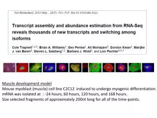
Muscle development model Mouse myoblast (muscle) cell line C2C12 induced to undergo myogenic differentiation. mRNA was isolated at : -24 hours, 60 hours, 120 hours, and 168 hours. Size selected fragments of approximately 200nt long for all of the time-points.

E N D
Muscle development model Mouse myoblast (muscle) cell line C2C12 induced to undergo myogenic differentiation. mRNA was isolated at : -24 hours, 60 hours, 120 hours, and 168 hours. Size selected fragments of approximately 200nt long for all of the time-points.
Some Differences with previous presentation 2010 vs 2008 Illumina 1G vs GAII transcriptomesequencing 430 million paired 75-bp reads vs 40 million single-end 25 bp reads Introduced TopHatvs introduce Cufflinks (uses TopHat) Detection of splice isoforms – RNAFAR vs Cufflinks: observation vs quantification Strong statistical framework FPKM : “expected number of fragments per kilobase of transcript sequence per millions base pairs sequenced”. Corresponds to transcript abundances (multiplied by a scalar). RPKM : “Reads per kilobase of exon model per million mapped reads”. (for single end experiments). Normalizes for RNA length and for the total read number in the measurement. Reflects the molar concentration in sample.
Summary of splicing related conclusions from previous talk Using TopHat: Identified ~17,000 candidate new parts of existing genes, but not in the gene models. Found evidence for 1.45 × 10⁵ different splices, from a library of ~2 × 10⁵ possible splices. TopHat does not require a reference transcriptome, so novel splice junctions could be found. Only looked for known alternative splice events. Did not attempt to quantify splice forms. Long-range contiguity of splice choices could not be extracted using single end reads. "Combining prevalence normalization of input RNA with paired-end sequencing would presumably give the most complete splicing pattern map." The tissue distribution of genes with two splice isoforms in the same tissue.
Questions Can we use RNA-seq to quantify isoform switching in a time series, at the level of: Differential promoter usage Differential splicing from a same TSS Issues Avoid the use of prior gene annotations Determination of fragment lengths Transcript abundance estimation Transcript assembly Analysis of Gene Expression Dynamics Goals Introduce Cufflinks Build a fully comprehensive map of splice isoforms Discover novel alternative transcription and splicing
1a- CuffLinks Input : mapped reads from an aligner The algorithm takes as input cDNA fragment sequences that have been aligned to the genome by software capable of producing spliced alignments, such as TopHat. With paired-end RNA-Seq, Cufflinks treats each pair of fragment reads as a single alignment. The algorithm assembles overlapping ‘bundles’ of fragment alignments separately, which reduces running time and memory use because each bundle typically contains the fragments from no more than a few genes. Now we need to assemble them
1b- CuffLinks Input : summary of mapping OK, Now we need to assemble them
2a- CuffLinks Assembly In the absence of an user provided annotation, Cufflinks assembles transcripts from alignments to the genome. Transcripts in each of the loci are assembled independently. The assembly algorithm is designed to aim for the following: (1) Every fragment is consistent with at least one assembled transcript. (2) Every transcript is tiled by reads. (3) The number of transcripts is the smallest required to satisfy requirement (1). (4) The resulting RNA-Seq models are "identifiable“ (ass below). In other words, we seek an assembly that parsimoniously explains the fragments from the RNA-Seq experiment; every fragment in the experiment should have come from a Cufflinks transcript, and Cufflinks should produce as few transcripts as possible with that property. Identifiability: L(ρ|R), where ρ is abundance, is the likelihood of a set of fragment alignments R.
Aside - Concept: Partial Order “A partially ordered set (or poset) formalizes and generalizes the intuitive concept of an ordering, sequencing, or arrangement of the elements of a set. A poset consists of a set together with a binary relation that indicates that, for certain pairs of elements in the set, one of the elements precedes the other. Such a relation is called a partial order to reflect the fact that not every pair of elements need be related: for some pairs, it may be that neither element precedes the other in the poset. A finite poset can be visualized through its Hasse diagram, which depicts the ordering relation.” Cufflinks constructs a partial order or equivalently a directed acyclic graph (DAG), with one node for each fragment that in turn consists of an aligned pair of mated reads. In the case of single reads, the partial order can be simply constructed by checking the reads for compatibility. In the case of paired-end RNA-Seq the situation is more complicated because of the unknown sequence between mate pairs.
1- Identify pairs of ‘incompatible’ fragments that must have originated from distinct spliced isoforms. 2- Connect compatible fragments in an ‘overlap graph’ where each fragment has one node in the graph, and an edge, directed from left to right along the genome, between each pair of ‘compatible’ fragments. 3- Assemble isoforms from the overlap graph by searching for paths through the graph corresponding to sets of mutually compatible fragments that could be merged into complete isoforms. 2b- CuffLinks Assembly Use Dilworth's theorem to produce a minimal set of paths that cover all the fragments in the overlap graph by finding the largest set of reads with the property that no two could have originated from the same isoform. Yellow, blue, and red fragments must have originated from separate isoforms, but any other fragment could have come from the same transcript as one of these three. The overlap graph here can be minimally ‘covered’ by three paths, each representing a different isoform.
Aside - Concept: Abundance FPKM is “expected number of fragments per kilobase of transcript sequence per millions base pairs sequenced”. Corresponds to transcript abundances (multiplied by a scalar). (compare to RPKM : “Reads per kilobase of exon model per million mapped reads”.) where adjusted transcript length F is the distribution of a random variable for actual fragment length. Thus,
THE BIG PICTURE – how to get these abundances R= set of aligned fragments ρ = relative abundance of different transcripts = {ρt}tЄT, T is the whole transcriptome. Σρt= 1 because they are relative abundances. We want to estimate them. Need to calculate the liklihood L(ρ|R) and maximize it. ρ = argmax [ L(ρ|R) ] F(i)= probability that a fragment has length i
MAXIMIZE THIS LIKLIHOOD Fragments are independent events, so the liklihood is the product of the probabilities for each “read alignment” Bayes Based on the assumption that transcripts are equally probable, normalized to length and abundance Portion of t in the mean Mean length of whole transcriptome Probthat we observe it exactly at this location= Prob the we observe a fragment of len It(r) Number of possible positions on t Len = It(r) F(i)= probability that we observe a fragment of length i =1 is the constraint r t
3- CuffLinks Abundance Estimation Fragments are matched to the transcripts from which they could have originated. Gray : could be from any of the three isoforms. Violet : could be from the blue or red isoform. Use fragment length distribution to assign fragments to isoforms. Thus, the violet fragment is more likely to be from the blue isoform than from the red isoform. Assume that probability of observing each fragment is a linear function of the abundances of the transcripts from which it could have originated. Numerically maximize a function that assigns a likelihood to all possible sets of relative abundances of the isoforms, producing the abundances that best explain the observed fragments. L(ρ|R), where ρ is abundance, is the likelihood of a set of fragment alignments R. It is equal to the product over all rЄR of the probabilities that a fragment selected at random originates from a given transcript .
Differential promoter usage versus splicing or other post-transcriptional regulation. Distinction of transcriptional and post-transcriptional regulatory effects on overall transcript output. When abundances of isoforms A, B, and C of Myc are grouped by TSS, changes in the relative abundances of the TSS groups indicate transcriptional regulation. Posttranscriptional effects are seen in changes in levels of isoforms of a single TSS group.
Aside - Concept: Overloading Transcripts that share a TSS are likely to be regulated by the same promoter, so tracking the change in relative abundances of groups of transcripts sharing a TSS may reveal how transcriptional regulation is affecting expression over time. “overloading” : a significant change in relative abundances for a set of transcripts. (In other words, isoform switching.) To quantify relative changes in expression in (groups of) transcripts, derive an entropy-based metric that can be used in a multiple hypothesis framework. The Jensen-Shannon divergence of a set of probability distributions is the entropy of their average minus the average of their entropies. It is symmetric and non-negative, and its square-root is a bona-fide "metric" (defines a distance between elements of a set). Test for overloaded genes by performing a one-sided t-test based on the asymptotics of the Jensen-Shannon metric under the null hypothesis of no change in relative abundnaces of isoforms. Type I errors were controlled with the Benjamini-Hochberg correction (FDR).
Isoforms of Myc have distinct expression dynamics. Myc isoforms are downregulated as the time course proceeds. Changes in relative abundances of Myc isoforms suggest that transcriptional effects immediately following differentiation at 0 hours give way to posttranscriptional effects later in the time course, as isoform A is eliminated.
MINARD PLOTS - For visualizing overloading and expression dynamics. Dotted line: gene level FPKM Black circles : measured FPKM Grey circles : mean of gene-level FPKM over consecutive time points Superimposes transcriptional and post-transcriptional overloading and gene level expression over the time course. The width of the colored band is the measure of change in relative transcript abundance and the color is the log ratio of transcriptional and post-transcriptional contributions to change in relative abundances
Fhl3 inhibits myogenesis by binding MyoD and attenuating its transcriptional activity A novel isoform for Fhl3 that is dominant during proliferation is supported by proximal TAF1 and RNA polymerase II ChIP-Seq peaks. The known isoform (solid line) is preferred at time points following differentiation.
Robustness of assembly and abundance estimation as a function of expression level and depth of sequencing. Subsets of the full 60-hour read set were mapped and assembled with TopHat and Cufflinks and the resulting assemblies were compared for structural and abundance agreement with the full 60 hour assembly. Colored lines show the results obtained at different depths of sequencing in the full assembly; e.g., the light blue line tracks the performance for transcripts with FPKM greater than 60. The fraction of transcript fragments fully recovered increases with additional sequencing data Abundance Estimates are similarly robust
Summary of Results Identified 7,770 genes and 10,480 isoforms undergoing significant abundance changes between some successive pair of time points (FDR < 5%). Many genes displayed switching between major and minor transcripts, some containing isoforms with muscle-specific functions. A total of 1,634 genes were found to have multiple isoforms with different trajectories in the time course. We hypothesized that differential promoter preference and differential splicing were responsible for the divergent patterns.