Download

1 / 54
620 likes | 1.54k Vues
Interpolation. Interpolation. Interpolation is important concept in numerical analysis. Quite often functions may not be available explicitly but only the values of the function at a set of points. . Interpolation. Interpolation is important concept in numerical analysis.

E N D
Interpolation • Interpolation is important concept in numerical analysis. • Quite often functions may not be available explicitly but only the values of the function at a set of points.
Interpolation • Interpolation is important concept in numerical analysis. • Quite often functions may not be available explicitly but only the values of the function at a set of points. • The values for f(xi) may be the results from a physical measurement (conductivity at different points around UWI)
Interpolation • It may also be from some long numerical calculation which can’t be put into a simple equation.
Interpolation • It may also be from some long numerical calculation which can’t be put into a simple equation. • What is required is that we estimate f(x)! i.e. Draw a smooth curve through xi.
Interpolation • The method of estimating between two known points (values) is called interpolation. • While estimating outside of know values is called extrapolation.
Interpolation • Interpolation is carried out using approximating functions such as: • Polynomials • Trigonometric functions • Exponential functions • Fourier methods
Interpolation Theory
Clearly a good approximation should be, such that the error between the true function and the approximation function should be very small.
Other than this approximating functions should have the following properties: • The function should be easy to determine • It should be easy to differentiate • It should be easy to evaluate • It should be easy to integrate
There are numerous theorems on the sorts of functions, which can be well approximated by which interpolating functions. • Generally these functions are of little use.
There are numerous theorems on the sorts of functions, which can be well approximated by which interpolating functions. • Generally these functions are of little use. • The following theorem is useful practically and theoretically for polynomial interpolation.
Weierstrass Approximation Theorem • If f(x) is a continuous real-valued function on [a, b] then for any > 0 , then there exists a polynomial Pn on [a, b] such that |ƒ(x) – Pn(x)| < for all x [a, b].
Weierstrass Approximation Theorem • This tells us that, any continuous function on a closed and bounded interval can be uniformly approximated on that interval by polynomial to any degree of accuracy. • However there is no guarantee that we will know f(x) to an accuracy for the theorem to hold.
Weierstrass Approximation Theorem • Consequently, any continuous function can be approximated to any accuracy by a polynomial of high enough degree.
Polynomial Approximation • Polynomials satisfy a uniqueness theorem: A polynomial of degree n passing exactly through n + 1 points is unique. • The polynomial through a specific set of points may take different forms, but all forms are equivalent. Any form can be manipulated into another form by simple algebraic rearrangement.
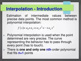
Polynomial Approximation • The Taylor series is a polynomial of infinite order. Thus ƒ(x) = ƒ(x0) + ƒ'(x0)(x - x0) + 1/2! ƒ''(x0) (x - x0)2+.. • However it is impossible computationally to evaluate an infinite number of terms.
Polynomial Approximation • Taylor polynomial of degree n is therefore usually defined as ƒ(x) = Pn(x) + Rn + 1(x) where the Taylor polynomial Pn(x) and the remainder term Rn + 1(x) are given by Pn(x) = ƒ(x0) + ƒ'(x0)(x - x0) + … + 1/n! ƒn(x0) (x - x0)n Rn + 1(x) = 1/(n+1)! ƒn+1( ξ ) (x - x0)n+1 where x0≤ξ<x.
Polynomial Approximation • The Taylor polynomial is a truncated Taylor series, with an explicit remainder, or error term. • The Taylor polynomial cannot be used as an approximating function for discrete data, because the derivatives required in the coefficients cannot be determined. • It does have great significance, however, for polynomial approximation because it has an explicit error term.
Polynomial Approximation • When a polynomial of degree n, Pn(x), is fitted exactly to a set of n + 1 discrete data points, (x0, f0), (x1, f1), …, (xn, fn), the polynomial has no error at the data points themselves. However, at the locations between the data points, there is an error, which is defined by E(x) = ƒ(x) - Pn(x) • This error term has the form E(x) = 1/(n+1)! (x - x0) (x – x1) … (x – xn) ƒn+1( ξ ); x0≤ξ≤x.
Interpolation In Practice
Interpolating Polynomials • Suppose we are given some values, the principle is that we fit a polynomial curve to the data. • The reason for this is that polynomials are well-behaved functions, requiring simple arithmetic calculations.
Interpolating Polynomials • Approximating polynomial (interpolating polynomial) should pass through all the known points. • Where it does not pass through the points it should be close to the function.
Interpolating Polynomials True function Approx 1 Approx 2 • Approximating polynomial (interpolating polynomial) should pass through all the known points. • Where it does not pass through the points it should be close to the function.
Interpolating Polynomials True function Approx 1 Approx 2 • Note that the interpolating polynomial may miss points of discontinuity. • There is only one interpolating polynomial P(xi) or less that matches the exact values; f(x0), f(x1),…, f(xn) at n+1 distinct base points.
Interpolating Polynomials Using Polynomials to approximate a function given discrete points
Interpolating Polynomials • We will be looking at two interpolating methods: • Lagrange Interpolation • Divided Difference
Lagrange Polynomials • A straightforward approach is the use of Lagrange polynomials. • The Lagrange Polynomial may be used where the data set is unevenly spaced.
Lagrange Polynomials • The formula used to interpolate between data pairs (x0,f(x0)), (x1,f(x1)),…, (xn,f(xn)) is given by, • Where the polynomial Pj(x) is given by,
Lagrange Polynomials • In general,
Lagrange Polynomials • Consider the table of interpolating points we wish to fit.
Lagrange Polynomials • The interpolation polynomial is,
Lagrange Polynomials • Note that the Lagrangian polynomial passes through each of the points used in its construction.
Advantages • The Lagrange formula is popular because it is well known and is easy to code. • Also, the data are not required to be specified with x in ascending or descending order.
Disadvantages • Although the computation of Pn(x) is simple, the method is still not particularly efficient for large values of n. • When n is large and the data for x is ordered, some improvement in efficiency can be obtained by considering only the data pairs in the vicinity of the x value for which Pn(x) is sought. • The price of this improved efficiency is the possibility of a poorer approximation to Pn(x).
Diagram showing Interpolation (incrementally from one to 5 points)
Newton’s Divided differences • The nth degree polynomial may be written in the special form:
Newton’s Divided differences • The nth degree polynomial may be written in the special form: • If we take ai such that Pn(x) = ƒ(x) at n+1 known points so that Pn(xi) = ƒ(xi), i=0,1,…,n, then Pn(x) is an interpolating polynomial.
Newton’s Divided differences • A divided difference is defined as the difference in the function values at two points, divided by the difference in the values of the corresponding independent variable. • Thus, the first divided difference at point is defined as
Newton’s Divided differences • Thus, the first divided difference at point is defined as • The second difference is given as: • In general,
Newton’s Divided differences • A divided difference table.
Newton’s Divided differences • One with actual values.
Newton’s Divided differences • The 3rd degree polynomial fitting all points from x0 = 3.2 to x3 = 4.8 is given by • P3(x) = 22.0 + 8.400(x - 3.2) + 2.856(x - 3.2)(x - 2.7) – 0.528(x - 3.2)(x - 2.7)(x - 1.0) • The 4th degree polynomial fitting all points is given by • P4(x) = P3(x) + 0.256(x - 3.2)(x - 2.7)(x - 1.0)(x - 4.8) • The interpolated value at x = 3.0 gives P3(x) = 20.2120.
Newton’s Divided differences • There are two disadvantages to using the Lagrangian interpolation polynomial for interpolation. • It involves more arithmetic operations than does the divided differences. 2. If we desire to add or subtract a point from the set to construct the polynomial, we essentially have to start over in the computations. The divided difference avoids this.
Newton’s Divided differences • Tabular data have a finite number of digits. The last digit is typically rounded off. Round off has an effect on the accuracy of the higher-order differences.