Download
1 / 41
530 likes | 846 Vues
computational geometry introduction. Mark de Berg. IPA Basic Course—Algorithms. introduction what is CG applications randomized incremental construction easy example: sorting a general framework applications to geometric problems and more …. Computational Geometry.

E N D
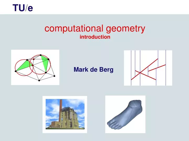
computational geometryintroduction Mark de Berg
IPA Basic Course—Algorithms introduction • what is CG • applications randomized incremental construction • easy example: sorting • a general framework • applications to geometric problems and more …
Computational Geometry Computational Geometry: Area within algorithms research dealing with spatial data (points, lines, polygons, circles, spheres, curves, … ) • design of efficient algorithms and data structures for spatial data • elementary operations are assumed to take O(1) time and be available focus on asymptotic running times of algorithms computing intersection point of two lines, distance between two points, etc
Map overlay annual rainfall land usage overlay
Computational Geometry example: compute all intersections in a set of line segments naïve algorithm fori= 1to n for j =i+1 ton doifsi intersects sj then report intersection Running time:O(n2) Can we do better ?
Computational geometry: applications (1) geographic information systems (GIS) Mississippi delta Arlington Arlington Memphis Memphis Memphis Memphis 30 cities: 430 = 1018 possibilities
Computational geometry: applications (2) computer-aided design and manufacturing (CAD/CAM) • motion planning • virtual walkthroughs 3D model of power plant (12.748.510 triangles)
9 5 4 6 8 7 3 2 1 Computational geometry: applications (3) 3D copier surface reconstruction 3D printer 3D scanner
Computational geometry: applications (4) • digitizing cultural heritage • custom-fit products • reverse engineering Other applications of surface reconstruction
Computational geometry: applications (5) • geographic information systems • computer-aided design and manufacturing • robotics and motion planning • computer graphics and virtual reality • databases • structural computational biology • and more … salary 50.000 30.000 30 45 age
Computational Geometry: algorithmic paradigms Deterministic algorithms • plane sweep • geometric divide-and-conquer Randomized algorithms • randomized incremental construction • random sampling today’s focus
EXERCISES • Let S be a set of n line segments in the plane. • Design an algorithm that decides in O (n log n) time if there are any intersections in S. Hint: Sort the endpoints on y-coordinates, and handle them in that order in a suitable manner. • Extend the algorithm so that it reports all intersections in time O ((n+k) log n), where k is the number of intersections. • For the experts: • Let u (n ) be the maximum number of pairs of points at distance 1 in a set of n points in the plane. Prove that u(n) =Ω (n log n). • Let D be a set of n discs in the plane. Prove that the union complexity of D is O (n ).
Plane-sweep algorithm for line-segment intersection • When two segments intersect, then there is a horizontal line L such that • the two segments both intersect L • they are neighbors along L sweep line insert segment 1 1 insert segment 2 insert segment 3 3 2 insert segment 4 insert segment 5 delete segment 1 4 5 6 Ordering along L: 1 1,2 3,1,2 3,1,4,2 3,5,1,4,2 3,5,4,2
Plane sweep SegmentIntersect • Sort the endpoints by y-coordinate. Let p1,…,p2n be the sorted set of endpoints. • Initialize empty search tree T. • fori = 1to2n • do { if piis the left endpoint of a segment s • then Insert s into thetree T • else Delete s from thetree T • Check all pairs of segments that become neighbors along the sweep line for intersection, report if there is an intersection. } Running time ? Extension to reporting all intersections ?
Lecture II: Randomized incremental construction Warm-up exercise: Analyze the worst-case and expected running time of the following algorithm. ParanoidMax (A) (* A [1..n ] is an array of n numbers *) • Randomly permute the elements in A • max := A[1] • fori := 2ton • do ifA [i ] > max • then { max := A[i ] • forj = 1toi -1 • do ifA[i ] > maxthen error } • returnmax
Worst-case running time Worst-case = O(1) + time for lines 2—7 = O(1) + ∑ 2≤i≤n (time for i-th iteration) = O(1) + ∑ 2≤i≤n ∑ 1≤j≤i-1 O(1) = O(1) + ∑ 2≤i≤n O(i) = O(n2)
Expected running time E [ looptijd ] = O(1) + E [ time for lines 2—7 ] = O(1) + E [ ∑ 2≤i≤n (time for i-th iteration) ] = O(1) + ∑ 2≤i≤n E [ time for i-th iteration ] = O(1) + ∑ 2≤i≤n { Pr [ A[i] ≤ max { A[1..i-1 ] } ] ∙ O(1) + Pr [ A[i] > max { A[1..i-1 ] } ] ∙ O(i) } = O(1) + ∑ 2≤i≤n { 1 ∙ O(1) + (1/i ) ∙ O(i) } = O(n )
EXERCISE • Give an algorithm that puts the elements of a given array A[1..n] into random order. Your algorithm should be such that every possible permutation is equally likely to be the result.
Sorting using Incremental Construction A geometric view of sorting Input: numbers x1,…,xn Output: partitioning of x-axis into a collection T of empty intervals defined by the input points x3 x1 x5 x4 x2 Incremental Construction: “Add” input points one by one, and maintain partitioning into intervals x3 x1 x5 x4 x2
Sorting using Incremental Construction • IC-Sort (S) • T := { [ -infty : +infty] } • fori := 1 to n • do { Findinterval J in T that contains xi and remove it. • Determine new intervals and insert them into T. } How? • for each point, maintain pointer to interval that contains it • for each interval in T, maintain conflict list of all points inside list: x4, x5 x3 x1 x5 x4 x2 list is empty
Sorting using Incremental Construction • IC-Sort (S) • T := { [ -infty : +infty] } • fori := 1 to n • do { Findinterval J in T that contains xi and remove it. • Determine new empty intervals and insert them into T. • Split conflict list of J to get the two new conflict lists. } • for each point, maintain pointer to interval that contains it • for each interval in T, maintain conflict list of all points inside Time analysis: TOTAL TIME: O ( total size of conflict lists of all intervals that ever appear) WORST-CASE: O(n2)
Sorting using Incremental Construction • RIC-Sort (S) • Randomly permute input points • T := { [ -infty : +infty] } • fori := 1 to n • do { Findinterval J in T that contains xi and remove it. • Determine new empty intervals and insert them into T. • Split conflict list of J to get the two new conflict lists. } • for each point, maintain pointer to interval that contains it • for each interval in T, maintain conflict list of all points inside Time analysis: TOTAL TIME: O ( total size of conflict lists of all intervals that are created) EXPECTED TIME: ??
An abstract framework for RIC S = set of n (geometric) objects; the input C= set of configurations D: assigns a defining set D(Δ) S to every configuration Δє C K: assigns a killing set K(Δ) S to every configuration ΔєC 4-tuple (S, C, D, K) is called a configuration space configurationΔє C is active over a subset S’ S if: D(Δ) S’ and K(Δ) S’ = o T(S) = active configurations over S; the output ∩ ∩ ∩ / ∩ ∩
Sorting using Incremental Construction • RIC(S) • Compute random permutation x1,…xn of input elements • T := { active configurations over empty set } • fori := 1 to n • do { Removeall configurations Δ with xi є K(Δ) from T. • Determine new active configurations; insert them into T. • Construct conflict lists of new active configurations. } • for each xi, maintain pointers to all configurations Δ such that xi є K(Δ) • for each configuration Δ in T, maintain conflict list of all xi є K(Δ) Theorem: Expected total size of conflict lists of all created configs: O( ∑ 1≤i≤n(n / i2) ∙ E [ # active configurations in step i ])
EXERCISE • Use the theorem to prove that the running time of the RIC algorithm for sorting runs in O( n log n ) time.
Lecture III RIC: more applications Voronoi diagrams and Delaunay triangulations
Principia Philosophiae (R. Descartes, 1644). The universe according to Descartes Voronoi diagram
. . . . . . . . . . . . . . . . . . . . . . . . . . . . . . . . . . . . . . . . . . . . . . . . . . . . . . . . . . . . . . . . . . . . . . . . . . . . . . . . . . . . . . . . . . . . . . . . . . . . . . . . . . . . . . . . . . . . . . . . . . . . . . . . . . . . . . . . . . . . . . . . . . . . . . . . . . . . . . . . . . . . . . . . . . . . . . . . . . . . . . . . . . . . . . . . . . . . . . . . . . . . . . . . . . . . . . . . . . . . . . . . . . . . . . . . . . . . . . . . . . . . . . . . . . . . . . . . . . . . . . . . . . . . . . . . . . . . . . . . . . 1163 1180 1153 1108 1127 981 1103 1098 1098 Construction of 3D height models (1) . . . . . . . . . . . . . . . . . . . . . . . . . . . . . . . . . . . . . . . . . . . . . . . . . . . . . . . . . . . . . . . . . . . . . . . . . . . . . . . . . . . . . . . . . . . . . . . . . . . . . . . . . . . . . . . . . . . . . . . . . . . . . . . . . . . . . . . . . . . . . . . . . . . . . . . . . . . . . . . . . . . . . . . . . . . . . . . . . . . . . . . . . . . . . . . . . . . . . . . . . . . . . . . . . . . . . . . . . . . . . . . . . . . . . . . . . . . . . . . . . . . . . . . . . . . . . . . . . . . . . . . . . . . . . . . . . . . . . . . . . . . . . . . . . . . . . . . . . . . . . . . . . . . . . . . . . . . . . . . . . . . . . . . . . . . . . . . . . . . . . . . . . . . . . . . . . . . . . . . . . . . . . . . . . . . . . . . . . . . . . . . . . . . . . . . . . . . . . . . . . . . . . . . . . . . . . . . . . . . . . . . . . . . . . . . . . . . . . . . . . . . . . . . . . . . . . . . . . . . . . . . . . . . . . . . . . . . . . . . . . . . . . . . . . . . . . . . . . . . . . . . . . . . . . . . . . . . . . . . . . . . . . . . . . . . . . . . . . . . . . . . . . . . . . . . . . . . . . . . . . . . . . . . . . . . . . . . . . . . . . . . . . . . . . . . . . . . . . . . . . . . . . . . . . . . . . . . . . . . . . . . . . . . . . . . . . . . . . . . . . . . . . . . . . . . . . . . . . . . . . . . . . . . . . . . . . . . . . . . . . . . . . . . . . . . . . . . . . . . . . . . . . . . . . . . . . . . . . . . . . . . . . . . . . . . . . . . . . . . . . . . . . . . . . . . . . . . . . . . . . . . . . . . . . . . . . . . . . . . . . . . . . . . . . . . . . . . . . . . . . . . . . . . . . . . . . . . . . . . . . . . . . . . . . . . . . . . . . . . . . . . . . . . . . . . . . . . . . . . . . . . . . . . . . . . . . . . . . . . . . . . . . . . . . . . . . . . . . . . . . . . . . . . . . . . . . . . . . . . . . . . . . . . . . . . . . . . . . . . . . . . . . . . . . . . . . . . . . . . . . . . . . . . . . . . . . .
Construction of 3D height models (2) 1163 1153 1180 1108 1127 1103 981 1098 1098 height?
Construction of 3D height models (3) Better: use interpolation to determine the height 983 983 triangulation
1163 1163 1153 1153 1180 1180 1108 1108 1127 1127 1103 1103 981 981 1098 1098 1098 1098 Construction of 3D height models (4) What is a good triangulation? long and thin triangles are bad try to avoid small angles
Construction of 3D height models (5) Voronoi diagram Delaunay triangulation: triangulation that maximizes the minimum angle !
Voronoi diagrams and Delaunay triangulations P : n points (sites) in the plane V(pi ) = Voronoi cell of site pi = { qєR2 : dist(q,pi ) < dist(q,pj ) for all j≠i } Vor(P ) = Voronoi diagram of P = subdivision induced by Voronoi cells DT(P) = Delaunay triangulation of P = dual graph of Vor(P)
EXERCISES • Prove: a triangle pipjpk is a triangle in DT(P) if and only if its circumcircle C (pipjpk ) does not contain any other site • Prove: number of triangles in DT(P) is at most2n-5 Hint: Euler’s formula for connected planar graphs: #vertices — #edges + #faces = 2 • Design and analyze a randomized incremental algorithm to construct DT(P).
RIC – Limitations of the framework Lecture IV: wrap-up Robot motion planning What is the region that is reachable for the robot?
RIC – Limitations of the framework (cont’d) The single-cell problem: Compute cell containing the origin Idea: compute vertical decomposition for the cell using RIC ?!
Spatial data structures more computational geometry • store geometric datain 2-, 3- or higher dimensional space such that certain queries can be answered efficiently • applications: GIS, graphics and virtual reality, … Examples: • point location • range searching • nearest-neighbor searching
and more … and more … • plane sweep • parametric search • arrangements • geometric duality, inversion, Plücker coordinates, … • kinetic data structures • core sets • Davenport-Schinzel sequences • …