Download
1 / 31
310 likes | 417 Vues
This paper introduces wavelet decompositions for data streams in streaming applications, utilizing one-pass algorithms and memory-efficient strategies. The proposed algorithm estimates wavelet coefficients using sketches, enabling real-time analysis of unbounded data. Learn about wavelet basics, Haar wavelet notation, sketch techniques, and sketch updating methods in the context of streaming data processing. Boost accuracy and confidence in approximating inner products and maintaining top coefficients using sketches.

E N D
One-Pass Wavelet Decompositions of Data Streams TKDE May 2002 Anna C. Gilbert,Yannis Kotidis, S. Muthukrishanan, Martin J. Strauss Presented by James Chan CSCI 599 Multidimensional Databases Fall 2003
Outline of Talk • Introduction • Background • Proposed Algorithm • Experiments • End Notes
Streaming Applications • Telephone Call Duration • Call Detail Record (CDR) • IP Traffic Flow • Bank ATM Transactions • Mission Critical Task: • Fraud • Security • Performance Monitoring
Data Stream Model Data Stream Problem • One Pass – no backtracking • Unbounded Data – Algorithms require small memory usage • Continuous – Need to run real time Synopsis in Memory Data Streams Stream Processing Engine (Approximate) Answer
Data Stream Strategies • Many stream algorithms produce approximate answers and have: • Deterministic Bounds: answers are within ± • Probabilistic Bounds: answers have high success probability (1-) within ±
Data Stream Strategies • Windows: New elements expire after time t • Samples: Approximate entire domain with a sample • Histograms: Partitioning element domain values into buckets (Equi-depth, V-Opt) • Wavelets: Haar, Construction and maintenance (difficult for large domain) • Sketch Techniques: estimate of L2 norm of a signal
Background: Cash Register vs. Aggregate • Cash Register: incoming stream represents domain (increment or decrement range of that domain) • Aggregate: incoming stream represents range, (update range of that domain) Note: Examples in this paper assume • each cash register element as +1 unit • no duplicate elements in aggregate models
Background: Wavelet Basics • Wavelet transforms capture trends in a signal • Typical transform involves log n passes • Each pass creates two sets of n/2 averages and differences. • Process repeated on averages • Output: Wavelet Basis vectors – one average and n-1 coefficients
Background: Haar Wavelet Notation • High pass filter • Low pass filter • Input: signal a • Basis Coefficients • Coefficients • Scaling Factor • Psi Vectors (un-normalized)
Most signals in nature have small B representation Only keep largest B wavelet coefficients to estimate energy of signal Additional coefficients do not help reduce squared sum error Background: Small B Representation Energy: SSE:
2.75 + -1.25 + 0.5 0 0 -1 0 -1 - + - + - + - + - + - + - 2 2 0 2 3 5 4 4 Original Signal Background: Storage • Highest B wavelet coefficients • Log N Straddling coefficients, one per level of the wavelet tree
Background: Bounding Theorems Theorem 1 • Given O(B+logN) storage (B is number of dimensions) • time to compute new data item is O(B+logN) in ordered aggregate model Theorem 2 • Any algorithm that calculates the 2nd largest wavelet coefficient of the signal in unordered CR / unordered agg uses at least N/polylog(N) • This holds if: • You only care about existence, not the coefficients value • Only calculating up to a factor of 2
Proposed Algorithm: Overview • Avoid keeping anything domain size N in memory • Estimate wavelet coefficients using sketches which are size log(N) • Sketch is maintained in memory and is updated as data entries stream in
What’s a Sketch? • Distortion Parameter (epsilon) • Failure Probability (delta) • Failure Threshold (eta) • Original Signal a • Random vector of {-1,+1}s r • Seed for r s • Atomic Sketch <a,r> dot product of a and r • Sketch O(log(N/ )/ ^2) atomic sketches • We use the same j to index the atomic sketch, seed, and random vector, so there are j atomic sketches in a sketch
Updating a Sketch • Cash Register • Add corresponding to the j atomic sketches • Aggregate • Add corresponding to the j atomic sketches • Use generator that takes in seed which is log(N) to compute
Reed Muller Generator {0} {d} {c} …. {d,c,b,a} • Pseudo random generator meeting these requirements: • Variables are 4 wise independent • Expected value of product of any 4 distinct r is 0 • Requires O(log N) space for seeding • Performs computation in polylog(N) time
Estimation of Inner Product O(log(1/)) X = median ( ) = mean ( ) … … O(log(1/^2)) … … …
… = means ( ) … Boosting Accuracy and Confidence • Improve accuracy to by averaging over more independent copies of for each average • Improve Confidence by increasing number of averages to take median over O(log(1/^2)) copies of … O(log(1/)) copies of … X = median of ( )
Using the sketches • We can approximate <a,> to maintain Bs • Note a point query is <a,ei> where e is a vector with a 1 at index i and 0s everywhere else Atomic Sketches in memory
Maintaining Top B Coefficients • At most Log N +1 coefficient updates • May need to approximate straddling coefficients to aggregate with already existing or near variables • Compare updates with top B and update top B if necessary updated unaffected
Algorithm Space and Time Their algorithm uses polylog(N) space and per item time to maintain B terms (by approximation)
Experiments • Data: one week of AT&T call detail (unordered cash register model) • Modes • Batch: Query only between intervals • Online: Query anytime • Direct Point: calc sketch of <ei,a> (ei is zero vector except with 1 at i) • Direct Wavelets: estimate all supporting coefficients and use wavelet reconstruction to calculate point a(i) • Top B: Reconstruction of point is done with Top B (maintained by sketch)
Top B - 1 Week (fixed-set) Value updates only. no replacement
Heavy Hitters • Points that contribute significantly to the energy of the signal • Direct point estimates are very accurate for heavy hitters but gross estimates for non heavy hitters • Adaptive Greedy pursuit: by removing the first heavy hitter from the signal, you improve the accuracy of calculating the next biggest heavy hitter • However an error is introduced with each subtraction of a heavy hitter
Processing Heavy Hitters Adaptive Greedy Pursuit
End Notes • First Provable Guarantees for haar wavelet over data streams • Can estimate Haar coefficients ci=<a,> • Top B is updated in: • This paper is superseded by "Fast, Small-space algorithms for approximatehistogram maintenance" STOC 2002 • Discusses how to select top B and find heavy hitters