Download
1 / 1
10 likes | 98 Vues
Comparison of SKA Survey Speeds John D. Bunton , CSIRO TIP. Introduction

E N D
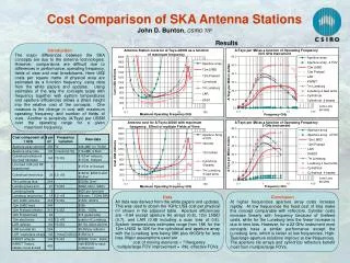
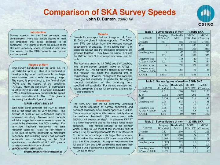
Comparison of SKA Survey SpeedsJohn D. Bunton, CSIRO TIP Introduction Survey speeds for the SKA concepts vary considerably. Here two simple figures of merit are proposed that allow concepts to be compared. The figures of merit are related to the sky and frequency space covered in unit time. The values for the SKA concepts are derived and compared. Results Results for concepts that can image at 1.4, 6 and 20 GHz are given in tables opposite. The FOVs and BWs are taken from the relevant concept descriptions or updates. In the tables both 12 m concepts (LNSD and the preloaded reflectors) are grouped together. They have the same FOV and the BW for the LNSD concept has been used for both. The Aperture array (at 1.4 GHz) and the Luneburg lens (in the current update) have an A/Tsys = 10,000 m2/K. This halves the sensitivity per image and requires four times the observing time to compensate. However, changes to the concepts could give full sensitivity. In particular, the original concept description of the Luneburg Lens specified full sensitivity. For the two concepts two values are given: one for full sensitivity and one for half sensitivity. Figures of Merit SKA survey bandwidth can be large e.g. HI for redshifts up to 4. Thus it is proposed to develop a figure of merit suitable for large area surveys over a wide frequency range. The speed is proportional to the field of view (FOV) and the square of the sensitivity (A/Tsys). Here the sensitivity (S) normalised to 20,00 m2/K is used. If concept bandwidth (BW) is less than survey bandwidth the speed is also proportional to BW. This gives a frequency bandwidth figure of merit: fbFOM = FOV x BW x S2 With wide band concepts the FOV at either end of the band can be very different. The overlap of fields at low frequencies leads to increased sensitivity. Narrow band concepts will take longer but some increase in speed is possible by eliminating the FOV overlap. For very low fractional bandwidth the time reduction factor is: TR(x)=1-x+1/3x2 where x is the ratio of survey bandwidth to maximum frequency. The resulting survey has constant sensitivity and normalising to the SKA specification bandwidth of 0.5 +f/5 give a constant sensitivity figure of merit: csFOM =FOV x BW xS2 x TR(BW/fmax)/TR(0.5/fmax+0.2) Discussion The 12m, LAR and the full sensitivity Luneburg lens, when operating at narrow bandwidth and constant sensitivity, have similar speeds at 1.4GHz. The aperture array is a little slower, mainly due to the restricted bandwidth (70 beams each with 200MHz, 44 beams per deg2). In all cases KARST is a slow instrument due to the single focus feeds specified. The fastest concept is the cylinder which is able to use most of the linefeed’s field of view (FOV) by trading bandwidth for FOV (factor of 6). A further advantage is its large filled aperture, which makes the correlator 15 times more efficient than the 12m concepts. At higher frequencies the full use of 12m and LAR bandwidths increases their relative FOM. However the cylinders is still about ten times faster.