Download
1 / 67
670 likes | 800 Vues
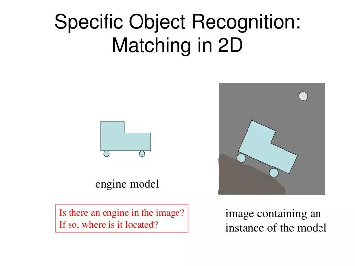
Specific Object Recognition: Matching in 2D. engine model. image containing an instance of the model. Is there an engine in the image? If so, where is it located?. Alignment. Use a geometric feature-based model of the object. Match features of the object to features in the image.

E N D
Specific Object Recognition: Matching in 2D engine model image containing an instance of the model Is there an engine in the image? If so, where is it located?
Alignment • Use a geometric feature-based model of the object. • Match features of the object to features in the image. • Produce a hypothesis h (matching features) • Compute an affine transformationT from h • Apply T to the features of the model to map the model features to the image. • Use a verification procedure to decide how well the model features line up with actual image features
Alignment model image
How can the object in the image differ from that in the model? Most often used: 2D Affine Transformations • translation • rotation • scale • skew
Point Representation and Transformations (review) Normal Coordinates for a 2D Point P = [x, y] = Homogeneous Coordinates P = [sx, sy, s] where s is a scale factor x y t t
Scaling x´ cx 0 x cx * x y´ 0 cy y cy * y = = scaling by a factor of 2 about (0,0)
Rotation x´ cos -sin x x cos - y sin y´ sin cos y x sin + y cos = = rotate point rotate axes
Translation 2 X 2 matrix doesn’t work for translation! Here’s where we need homogeneous coordinates. x´ 1 0 x0 x x + x0 y´ 0 1 y0 y y + y0 1 0 0 1 1 1 = = (x+x0, y + y0) (x,y)
Rotation, Scaling and Translation xw 1 0 x0 s 0 0 cos -sin 0 xi yw = 0 1 y0 0 s 0 sin cos 0 yi 1 0 0 1 0 0 1 0 0 1 1 T S R TR
Computing Affine Transformations between Sets of Matching Points P2=(x2,y2) P3´=(u3,v3) P2´=(u2,v2) P1´=(u1,v1) P1=(x1,y1) P3=(x3,y3) Given 3 matching pairs of points, the affine transformation can be computed through solving a simple matrix equation. u1 u2 u3a11 a12 a13 x1 x2 x3 v1 v2 v3 = a21 a22 a23 y1 y2 y3 1 1 1 0 0 1 1 1 1
A More Robust Approach Using only 3 points is dangerous, because if even one is off, the transformation can be far from correct. Instead, use many (n =10 or more) pairs of matching control points to determine a least squares estimate of the six parameters of the affine transformation. Error(a11, a12, a13, a21, a22, a23) = ((a11*xj + a12*yj + a13 - uj)2 + (a21*xj + a22*yj + a23 - vj)2 ) j=1,n
What is this for? • Many 2D matching techniques use it. • 1. Local-Feature Focus Method • 2. Pose Clustering • 3. Geometric Hashing
Local-Feature-Focus Method • Each model has a set of features (interesting points). • -The focus features are the particularly detectable features, • usually representing several different areas of the model. • - Each focus feature has a set of nearby features that • can be used, along with the focus feature, to compute • the transformation. focus feature
LFF Algorithm Let G be the set of detected image features. Let Fm be focus features of the model. Let S(f) be the nearby features for feature f. for each focus feature Fm for each image feature Gi of the same type as Fm 1. find the maximal subgraph Sm of S(Fm) that matches a subgraph Si of S(Gi). 2. Compute transformation T that maps the points of each feature of Sm to the corresponding one of Si. 3. Apply T to the line segments of the model. 4. If enough transformed segments find evidence in the image, return(T)
Example Match 1: Good Match G1 F1 F3 F4 F2 G4 G2 G3
Example Match 2: Poor Match G5 E1 E3 E4 E2 G8 G6 G7
Pose Clustering Let T be a transformation aligning model M with image object O The pose of object O is its location and orientation, defined byT. The idea of pose clustering is to compute lots of possible pose transformations, each based on 2 points from the model and 2 hypothesized corresponding points from the image.* Then cluster all the transformations in pose space and try to verify the large clusters. * This is not a full affine transformation, just RST.
Pose Clustering Model Image
Pose Clustering Model Image
Geometric Hashing • This method was developed for the case where there is • a whole database of models to try to find in an image. • It trades: • a large amount of offline preprocessing and • a large amount of space • for potentially fast online • object recognition • pose detection
Theory Behind Geometric Hashing • A model M is a an ordered set of feature points. 3 1 2 M = <P1,P2,P3,P4,P5,P6,P7,P8> 8 4 6 7 5 • An affine basis is any subset E={e00,e01,e10} • of noncollinear points of M. • For basis E, any point x M can be represented in • affine coordinates(,). • x = (e10 – e00) + (e01-e00) + e00 e01 x = (,) e10 e00
Affine Transform If x is represented in affine coordinates (,). x = (e10 – e00) + (e01- e00) + e00 and we apply affine transform T to point x, we get Tx =(Te10 – Te00) + (Te01-Te00) + Te00 In both cases, x has the same coordinates (,).
Example transformed object original object
Offline Preprocessing For each model M { Extract feature point set FM for each noncollinear triple E of FM (basis) for each other point x of FM { calculate (,) for x with respect to E store (M,E) in hash table H at index (,) } }
Hash Table list of model / basis pairs M1, E1 M2, E2 . . Mn, En
E1 … Em Online Recognition M1 . . initialize accumulator A to all zero extract feature points from image for each basis triple F/* one basis */ for each other point v /* each image point */ { calculate (,) for v with respect to F retrieve list L from hash table at index (,) for each pair (M,E) of L A[M,E] = A[M,E] + 1 } find peaks in accumulator array A for each peak (M,E) in A calculate and try to verify T : F = TE Mk (M,E)->T
Molecular Biology ExampleTel Aviv UniversityProtein Matching
Verification How well does the transformed model line up with the image. Whole segments work better, allow less halucination, but there’s a higher cost in execution time. • compare positions of feature points • compare full line or curve segments
2D Matching Mechanisms • We can formalize the recognition problem as finding • a mapping from model structures to image structures. • Then we can look at different paradigms for solving it. - interpretation tree search - discrete relaxation - relational distance - continuous relaxation
Formalism • A part (unit) is a structure in the scene, • such as a region or segment or corner. • A label is a symbol assigned to identify the part. • An N-ary relation is a set of N-tuples defined over a • set of parts or a set of labels. • An assignment is a mapping from parts to labels.
Example image model circle4 circle5 arc1 eye1 eye2 circle1 head circle2 smile circle3 What are the relationships? What is the best assignment of model labels to image features?
Consistent Labeling Definition Given: 1. a set of units P 2. a set of labels for those units L 3. a relation RP over set P 4. a relation RL over set L A consistent labeling f is a mapping f: P -> L satisfying if (pi, pj) RP, then (f(pi), f(pj)) RL which means that a consistent labeling preserves relationships.
Abstract Example binary relation RL b binary relation RP c 1 a 2 3 d e P = {1,2,3} L = {a,b,c,d,e} RP={(1,2),(2,1),(2,3)} RL = {(a,c),(c,a),(c,b), (c,d),(e,c),(e,d)} One consistent labeling is {(1,a),(2,c),(3,d)
House Example P L RP and RL are connection relations. f(S1)=Sj f(S2)=Sa f(S3)=Sb f(S4)=Sn f(S5)=Si f(S6)=Sk f(S10)=Sf f(S11)=Sh f(S7)=Sg f(S8) = Sl f(S9)=Sd
1. Interpretation Tree • An interpretation tree is a tree that represents all • assignments of labels to parts. • Each path from the root node to a leaf represents • a (partial) assignment of labels to parts. • Every path terminates as either • 1. a complete consistent labeling • 2. a failed partial assignment
Interpretation Tree Example b RP 1 2 RL a c 3 root e d … (1,a) (2,b) (2,c) … X (3,b) (3,d) (3,e) (1,2) RP (a,b) RL X OK OK
2. Discrete Relaxation • Discrete relaxation is an alternative to (or addition to) • the interpretation tree search. • Relaxation is an iterative technique with polynomial • time complexity. • Relaxation uses local constraints at each iteration. • It can be implemented on parallel machines.
How Discrete Relaxation Works 1. Each unit is assigned a set of initial possible labels. 2. All relations are checked to see if some pairs of labels are impossible for certain pairs of units. 3. Inconsistent labels are removed from the label sets. 4. If any labels have been filtered out then another pass is executed else the relaxation part is done. 5. If there is more than one labeling left, a tree search can be used to find each of them.
Example of Discrete Relaxation RP RL L1 L2 L3 Pi L1 L2 L3 X L8 L6 Pj L6 L8 There is no label in Pj’s label set that is connected to L2 in Pi’s label set. L2 is inconsistent and filtered out.
3. Relational Distance Matching • A fully consistent labeling is unrealistic. • An image may have missing and extra features; • required relationships may not always hold. • Instead of looking for a consistent labeling, • we can look for the best mapping from P to L, • the one that preserves the most relationships. b 1 2 a c 3
Preliminary Definitions Def: A relational description DP is a sequence of relations over a set of primitives P. • Let DA = {R1,…,RI} be a relational description over A. • Let DB = {S1,…,SI} be a relational description over B. • Let f be a 1-1, onto mapping from A to B. • For any relation R, the composition Rf is given by • Rf = {(b1,…,bn) | (a1,…,an) is in R and f(ai)=(bi), i=1,n}
Example of Composition Rf = {(b1,…,bn) | (a1,…,an) is in R and f(ai)=(bi), i=1,n} b 1 2 1 a 2 b 3 c a c 3 f R Rf Rf is an isomorphic copy of R with nodes renamed by f.
Relational Distance Definition Let DA be a relational description over set A, DB be a relational description over set B, and f : A -> B. • The structural error of f for Ri in DA and Si in DB is • E (f) = | Ri f - Si | + | Si f - Ri | • The total error of f with respect to DA and DB is • E(f) = E (f) • The relational distance GD(DA,DB) is given by • GD(DA,DB) = min E(f) -1 i S I i S i=1 f : A B, f is 1-1 and onto
Example a b 1 2 3 4 c d What is the best mapping? What is the error of the best mapping?
ExampleLet f = {(1,a),(2,b),(3,c),(4,d)} a b 1 2 S R 3 4 c d | Rf - S | = |{(a,b)(b,c)(c,d)(d,b)} - {(a,b)(b,c)(c,b)(d,b)} | = |{(c,d)}| = 1 -1 |S f - R | = |{(1,2)(2,3)(3,2)(4,2)} - {(1,2)(2,3)(3,4)(4,2)}| = |{(3,2)}| = 1 Is there a better mapping? E(f) = 1+1 = 2