Download
1 / 71
720 likes | 913 Vues
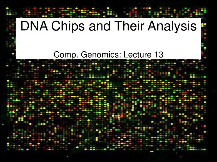
DNA Chips and Their Analysis Comp. Genomics: Lecture 13. What is a DNA Microarray?. An experiment on the order of 10k elements A way to explore the function of a gene A snapshot of the expression level of an entire phenotype under given test conditions . Some Microarray Terminology.

E N D
What is a DNA Microarray? • An experiment on the order of 10k elements • A way to explore the function of a gene • A snapshot of the expression level of an entire phenotype under given test conditions
Some Microarray Terminology • Probe: ssDNA printed on the solid substrate (nylon or glass) These are the genes we are going to be testing • Target: cDNA which has been labeled and is to be washed over the probe
Microarray Fabrication • Deposition of DNA fragments • Deposition of PCR-amplified cDNA clones • Printing of already synthesized oligonucleotieds • In Situ synthesis • Photolithography • Ink Jet Printing • Electrochemical Synthesis From “Data Analysis Tools for DNA Microarrays” by Sorin Draghici
cDNA Microarrays and Oligonucleotide Probes From “Data Analysis Tools for DNA Microarrays” by Sorin Draghici
In Situ Synthesis • Photochemically synthesized on the chip • Reduces noise caused by PCR, cloning, and Spotting • As previously mentioned, three kinds of In Situ Synthesis • Photolithography • Ink Jet Printing • Electrochemical Synthesis From “Data Analysis Tools for DNA Microarrays” by Sorin Draghici
Photolithography • Similar to process used to build VLSI circuits • Photolithographic masks are used to add each base • If base is present, there will be a hole in the corresponding mask • Can create high density arrays, but sequence length is limited Photodeprotection mask C From “Data Analysis Tools for DNA Microarrays” by Sorin Draghici
Ink Jet Printing • Four cartridges are loaded with the four nucleotides: A, G, C,T • As the printer head moves across the array, the nucleotides are deposited where they are needed From “Data Analysis Tools for DNA Microarrays” by Sorin Draghici
Electrochemical Synthesis • Electrodes are embedded in the substrate to manage individual reaction sites • Electrodes are activated in necessary positions in a predetermined sequence that allows the sequences to be constructed base by base • Solutions containing specific bases are washed over the substrate while the electrodes are activated From “Data Analysis Tools for DNA Microarrays” by Sorin Draghici
Color Coding • Tables are difficult to read • Data is presented with a color scale • Coding scheme: • Green = repressed (less mRNA) gene in experiment • Red = induced (more mRNA) gene in experiment • Black = no change (1:1 ratio) • Or • Green = control condition (e.g. aerobic) • Red = experimental condition (e.g. anaerobic) • We only use ratio Campbell & Heyer, 2003
Application of Microarrays • We only know the function of about 20% of the 30,000 genes in the Human Genome • Gene exploration • Faster and better • Can be used for DNA computing http://www.gene-chips.com/sample1.html From “Data Analysis Tools for DNA Microarrays” by Sorin Draghici
A Data Mining Problem • On a given Microarray we test on the order of 10k elements at a time • Data is obtained faster than it can be processed • We need some ways to work through this large data set and make sense of the data
Example data: fold change (ratios) What is the pattern? Campbell & Heyer, 2003
Example data: log2 transformation Campbell & Heyer, 2003
Pearson Correlation Coefficient, rvalues in [-1,1] interval • Gene expression over time is a vector, e.g. for gene C: (0, 3, 3.58, 4, 3.58, 3) • Given two vectors X and Y that contain N elements, we calculate r as follows: Cho & Won, 2003
Pearson Correlation Coefficient, r (cont.) • X = Gene C = (0, 3.00, 3.58, 4, 3.58, 3)Y = Gene D = (0, 1.58, 2.00, 2, 1.58, 1) • ∑XY = (0)(0)+(3)(1.58)+(3.58)(2)+(4)(2)+(3.58)(1.58)+(3)(1) = 28.5564 • ∑X = 3+3.58+4+3.58+3 = 17.16 • ∑X2 = 32+3.582+42+3.582+32 = 59.6328 • ∑Y = 1.58+2+2+1.58+1 = 8.16 • ∑Y2 = 1.582+22+22+1.582+12 = 13.9928 • N = 6 • ∑XY – ∑X∑Y/N = 28.5564 – (17.16)(8.16)/6 = 5.2188 • ∑X2 – (∑X)2/N = 59.6328 – (17.16)2/6 = 10.5552 • ∑Y2 – (∑Y)2/N = 13.9928 – (8.16)2/6 = 2.8952 • r = 5.2188 / sqrt((10.5552)(2.8952)) = 0.944
Example data: Pearson correlation coefficient Campbell & Heyer, 2003
Example: Reorganization of data Campbell & Heyer, 2003
Pearson Rank Correlation Coefficient • Replace each entry xi by its rank in vector x. • Then compute Pearson correlation coefficients of rank vectors. • Example: X = Gene C = (0, 3.00, 3.41, 4, 3.58, 3.01) Y = Gene D = (0, 1.51, 2.00, 2.32, 1.58, 1) • Ranks(X)= (1,2,4,6,5,3) • Ranks(Y)= (1,3,5,6,4,2) • Ties should be taken care of: (1) rare (2) randomize (small effect)
Grouping and Reduction • Grouping: discovers patterns in the data from a microarray • Reduction: reduces the complexity of data by removing redundant probes (genes) that will be used in subsequent assays
Unsupervised Grouping: Clustering • Pattern discovery via grouping similarly expressed genes together • Techniques most often used • k-Means Clustering • Hierarchical Clustering • Biclustering • Additional Methods: Self Organizing Maps (SOMS), plaid models, singular value decomposition (SVD), order preserving submatrices (OPSM),……
Clustering Overview • Different similarity measures • Pearson Correlation Coefficient • Cosine Coefficient • Euclidean Distance • Information Gain • Mutual Information • Signal to noise ratio • Simple Matching for Nominals
Clustering Overview (cont.) • Different Clustering Methods • Unsupervised • k-means Clustering (k nearest neighbors) • Hierarchical Clustering • Self-organizing map • Supervised • Support vector machine • Ensemble classifier • Data Mining
Clustering Limitations • Any data can be clustered, therefore we must be careful what conclusions we draw from our results • Clustering is often randomized and can and will produce different results for different runs on same data
K-means Clustering • Given a set of m data points in n-dimensional space and an integer k • We want to find the set of k points in n-dimensional space that minimizes the Euclidean (mean squared) distance from each data point to its nearest center • No exact polynomial-time algorithms are known for this problem (no wonder, NP-hard!) “A Local Search Approximation Algorithm for k-Means Clustering” by Kanungo et. al
K-means Heuristic (Lloyd’s Algorithm) • Has been shown to converge to a locally optimal solution • But can converge to a solution arbitrarily bad compared to the optimal solution Data Points Optimal Centers Heuristic Centers K=3 • “K-means-type algorithms: A generalized convergence theorem and characterization of local optimality” by Selim and Ismail • “A Local Search Approximation Algorithm for k-Means Clustering” by Kanungo et al.
Euclidean Distance Now to find the distance between two points, say the origin and the point (3,4): Simple and Fast! Remember this when we consider the complexity!
Finding a Centroid We use the following equation to find the n dimensional centroid point (center of mass) amid k (n dimensional) points: Example: Let’s find the midpoint between three 2D points, say: (2,4) (5,2) (8,9)
K-means Iterative Heuristic • Choose k initial center points “randomly” • Cluster data using Euclidean distance (or other distance metric) • Calculate new center points for each cluster, using only points within the cluster • Re-Clusterall data using the new center points (this step could cause some data points to be placed in a different cluster) • Repeat steps 3 & 4 until no data points are moved from one cluster to another (stabilization), or till some other convergence criteria is met From “Data Analysis Tools for DNA Microarrays” by Sorin Draghici
An example with 2 clusters • We Pick 2 centers at random • We cluster our data around these center points Figure Reproduced From “Data Analysis Tools for DNA Microarrays” by Sorin Draghici
K-means example with k=2 • We recalculate centers based on our current clusters Figure Reproduced From “Data Analysis Tools for DNA Microarrays” by Sorin Draghici
K-means example with k=2 • We re-cluster our data around our new center points Figure Reproduced From “Data Analysis Tools for DNA Microarrays” by Sorin Draghici
K-means example with k=2 5. We repeat the last two steps until no more data points are moved into a different cluster Figure Reproduced From “Data Analysis Tools for DNA Microarrays” by Sorin Draghici
Choosing k • Run algorithm on data with several different values of k • Use advance knowledge about the characteristics of your test (e.g. Cancerous vs Non-Cancerous Tissues, in case the experiments are being clustered)
Cluster Quality • Since any data can be clustered, how do we know our clusters are meaningful? • The size (diameter) of the cluster vs. the inter-cluster distance • Distance between the members of a cluster and the cluster’s center • Diameter of the smallest sphere containing the cluster From “Data Analysis Tools for DNA Microarrays” by Sorin Draghici
Cluster Quality Continued distance=5 diameter=5 distance=20 Quality of cluster assessed by ratio of distance to nearest cluster and cluster diameter diameter=5 Figure Reproduced From “Data Analysis Tools for DNA Microarrays” by Sorin Draghici
Cluster Quality Continued Quality can be assessed simply by looking at the diameter of a cluster (alone????) A cluster can be formed by the heuristic even when there is no similarity between clustered patterns. This occurs because the algorithm forces k clusters to be created. From “Data Analysis Tools for DNA Microarrays” by Sorin Draghici
Characteristics of k-means Clustering • The random selection of initial center points creates the following properties • Non-Determinism • May produce clusters without patterns • One solution is to choose the centers randomly from existing patterns From “Data Analysis Tools for DNA Microarrays” by Sorin Draghici
Heuristic’s Complexity • Linear in the number of data points, N • Can be shown to have run time cN, where c does not depend on N, but rather the number of clusters, k • (not sure about dependence on dimension, n?) heuristic is efficient From “Data Analysis Tools for DNA Microarrays” by Sorin Draghici
Hierarchical Clustering • a different clustering paradigm Figure Reproduced From “Data Analysis Tools for DNA Microarrays” by Sorin Draghici
Hierarchical Clustering (cont.) Campbell & Heyer, 2003
Hierarchical Clustering (cont.) C • Average “similarity” to • Gene D: (0.94+0.84)/2 = 0.89 • Gene F: (-0.40+(-0.57))/2 = -0.485 • Gene G: (0.95+0.89)/2 = 0.92 1 D E F 1 G C E
Hierarchical Clustering (cont.) 1 2 D C E G D F G
Hierarchical Clustering (cont.) 3 1 2 C E G D F
Hierarchical Clustering (cont.) 4 3 F 1 2 F C E G D
Hierarchical Clustering (cont.) algorithm looks familiar? 4 Remember Neighbor-Joining ! 3 1 2 F C E G D
Clustering of entire yeast genome Campbell & Heyer, 2003
Hierarchical Clustering:Yeast Gene Expression Data Eisen et al., 1998
A SOFM Example With Yeast “Interpresting patterns of gene expression with self-organizing maps: Methods and application to hematopoietic differentiation” by Tamayo et al.