Download
1 / 47
480 likes | 674 Vues
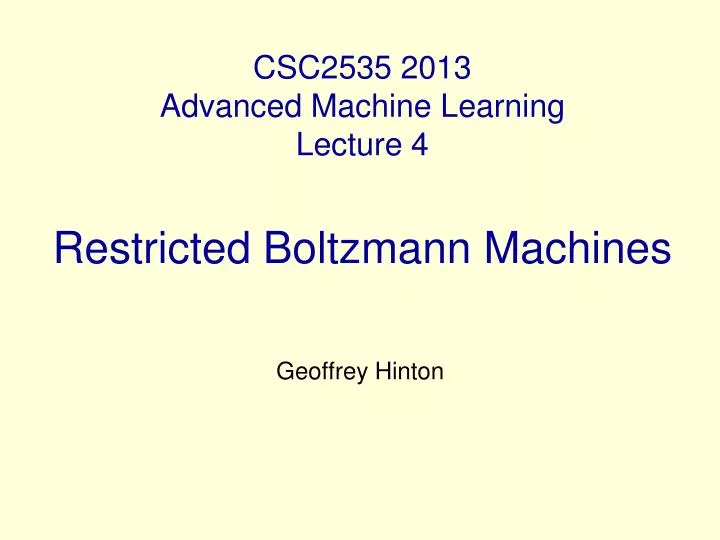
CSC2535 2013 Advanced Machine Learning Lecture 4 Restricted Boltzmann Machines. Geoffrey Hinton. Three ways to combine probability density models. Mixture: Take a weighted average of the distributions.

E N D
CSC2535 2013Advanced Machine LearningLecture 4Restricted Boltzmann Machines Geoffrey Hinton
Three ways to combine probability density models • Mixture: Take a weighted average of the distributions. • It can never be sharper than the individual distributions. It’s a very weak way to combine models. • Product: Multiply the distributions at each point and then renormalize (this is how an RBM combines the distributions defined by each hidden unit) • Exponentially more powerful than a mixture. The normalization makes maximum likelihood learning difficult, but approximations allow us to learn anyway. • Composition: Use the values of the latent variables of one model as the data for the next model. • Works well for learning multiple layers of representation, but only if the individual models are undirected.
Two types of generative neural network • If we connect binary stochastic neurons in a directed acyclic graph we get a Sigmoid Belief Net (Radford Neal 1992). • If we connect binary stochastic neurons using symmetric connections we get a Boltzmann Machine (Hinton & Sejnowski, 1983). • If we restrict the connectivity in a special way, it is easy to learn a Boltzmann machine.
Restricted Boltzmann Machines(Smolensky ,1986, called them “harmoniums”) hidden • We restrict the connectivity to make learning easier. • Only one layer of hidden units. • We will deal with more layers later • No connections between hidden units. • In an RBM, the hidden units are conditionally independent given the visible states. • So we can quickly get an unbiased sample from the posterior distribution when given a data-vector. • This is a big advantage over directed belief nets j i visible
The Energy of a joint configuration(ignoring terms to do with biases) binary state of visible unit i binary state of hidden unit j Energy with configuration v on the visible units and h on the hidden units weight between units i and j
A picture of the maximum likelihood learning algorithm for an RBM j j j j a fantasy i i i i t = 0 t = 1 t = 2 t = infinity Start with a training vector on the visible units. Then alternate between updating all the hidden units in parallel and updating all the visible units in parallel.
A quick way to learn an RBM Start with a training vector on the visible units. Update all the hidden units in parallel Update the all the visible units in parallel to get a “reconstruction”. Update the hidden units again. j j i i t = 0 t = 1 reconstruction data This is not following the gradient of the log likelihood. But it works well. It is approximately following the gradient of another objective function (Carreira-Perpinan & Hinton, 2005).
Collaborative filtering: The Netflix competition • You are given most of the ratings that half a million Users gave to 18,000 Movies on a scale from 1 to 5. • Each user only rates a small fraction of the movies. • You have to predict the ratings users gave to the held out movies. • If you win you get $1000,000
Lets use a “language model” rating The data is strings of triples of the form: User, Movie, rating. U2 M1 5 U2 M3 1 U4 M1 4 U4 M3 ? All we have to do is to predict the next “word” well and we will get rich. M3 feat scalar product U4 feat 3.1 U4 feat M3 feat U4 M3 matrix factorization
An RBM alternative to matrix factorization • Suppose we treat each user as a training case. • A user is a vector of movie ratings. • There is one visible unit per movie and its a 5-way softmax. • The CD learning rule for a softmax is the same as for a binary unit. • There are ~100 hidden units. • One of the visible values is unknown. • It needs to be filled in by the model. about 100 binary hidden units M1 M2 M3 M4 M5 M6 M7 M8
How to avoid dealing with all those missing ratings • For each user, use an RBM that only has visible units for the movies the user rated. • So instead of one RBM for all users, we have a different RBM for every user. • All these RBMs use the same hidden units. • The weights from each hidden unit to each movie are shared by all the users who rated that movie. • Each user-specific RBM only gets one training case! • But the weight-sharing makes this OK. • The models are trained with CD1 then CD3, CD5 & CD9.
How well does it work?(Salakhutdinov et al. 2007) • RBMs work about as well as matrix factorization methods, but they give very different errors. • So averaging the predictions of RBMs with the predictions of matrix-factorization is a big win. • The winning group used multiple different RBM models in their average of over a hundred models. • Their main models were matrix factorization and RBMs.
An improved version of Contrastive Divergence learning • The main worry with CD is that there will be deep minima of the energy function far away from the data. • To find these we need to run the Markov chain for a long time (maybe thousands of steps). • But we cannot afford to run the chain for too long for each update of the weights. • Maybe we can run the same Markov chain over many weight updates? (Neal, 1992) • If the learning rate is very small, this should be equivalent to running the chain for many steps and then doing a bigger weight update.
Persistent CD(Tijmen Teileman, ICML 2008 & 2009) • Use minibatches of 100 cases to estimate the first term in the gradient. Use a single batch of 100 fantasies to estimate the second term in the gradient. • After each weight update, generate the new fantasies from the previous fantasies by using one alternating Gibbs update. • So the fantasies can get far from the data.
Contrastive divergence as an adversarial game • Why does persisitent CD work so well with only 100 negative examples to characterize the whole partition function? • For all interesting problems the partition function is highly multi-modal. • How does it manage to find all the modes without starting at the data?
The learning causes very fast mixing • The learning interacts with the Markov chain. • Persisitent Contrastive Divergence cannot be analysed by viewing the learning as an outer loop. • Wherever the fantasies outnumber the positive data, the free-energy surface is raised. This makes the fantasies rush around hyperactively.
How persistent CD moves between the modes of the model’s distribution • If a mode has more fantasy particles than data, the free-energy surface is raised until the fantasy particles escape. • This can overcome free-energy barriers that would be too high for the Markov Chain to jump. • The free-energy surface is being changed to help mixing in addition to defining the model.
Modeling real-valued data • For images of digits it is possible to represent intermediate intensities as if they were probabilities by using “mean-field” logistic units. • We can treat intermediate values as the probability that the pixel is inked. • This will not work for real images. • In a real image, the intensity of a pixel is almost always almost exactly the average of the neighboring pixels. • Mean-field logistic units cannot represent precise intermediate values.
A standard type of real-valued visible unit • We can model pixels as Gaussian variables. Alternating Gibbs sampling is still easy, though learning needs to be much slower. E energy-gradient produced by the total input to a visible unit parabolic containment function Welling et. al. (2005) show how to extend RBM’s to the exponential family. See also Bengio et. al. (2007)
Gaussian-Binary RBM’s • Lots of people have failed to get these to work properly. Its extremely hard to learn tight variances for the visible units. • It took a long time for us to figure out why it is so hard to learn the visible variances. • When sigma is small, we need many more hidden units than visible units. • This allows small weights to produce big top-down effects. When sigma is much less than 1, the bottom-up effects are too big and the top-down effects are too small.
Replacing binary variables by integer-valued variables(Teh and Hinton, 2001) • One way to model an integer-valued variable is to make N identical copies of a binary unit. • All copies have the same probability, of being “on” : p = logistic(x) • The total number of “on” copies is like the firing rate of a neuron. • It has a binomial distribution with mean N p and variance N p(1-p)
A better way to implement integer values • Make many copies of a binary unit. • All copies have the same weights and the same adaptive bias, b, but they have different fixed offsets to the bias:
A fast approximation • Contrastive divergence learning works well for the sum of binary units with offset biases. • It also works for rectified linear units. These are much faster to compute than the sum of many logistic units. output = max(0, x + randn*sqrt(logistic(x)) )
How to train a bipartite network of rectified linear units • Just use contrastive divergence to lower the energy of data and raise the energy of nearby configurations that the model prefers to the data. Start with a training vector on the visible units. Update all hidden units in parallel with sampling noise Update the visible units in parallel to get a “reconstruction”. Update the hidden units again j j i i reconstruction data
3D Object Recognition: The NORB dataset Stereo-pairs of grayscale images of toy objects. Animals Humans Normalized-uniform version of NORB Planes Trucks Cars - 6 lighting conditions, 162 viewpoints • Five object instances per class in the training set • A different set of five instances per class in the test set - 24,300 training cases, 24,300 test cases
Simplifying the data • Each training case is a stereo-pair of 96x96 images. • The object is centered. • The edges of the image are mainly blank. • The background is uniform and bright. • To make learning faster I used simplified the data: • Throw away one image. • Only use the middle 64x64 pixels of the other image. • Downsample to 32x32 by averaging 4 pixels.
Simplifying the data even more so that it can be modeled by rectified linear units • The intensity histogram for each 32x32 image has a sharp peak for the bright background. • Find this peak and call it zero. • Call all intensities brighter than the background zero. • Measure intensities downwards from the background intensity. 0
Test set error rates on NORB after greedy learning of one or two hidden layers using rectified linear units Full NORB (2 images of 96x96) • Logistic regression on the raw pixels 20.5% • Gaussian SVM (trained by Leon Bottou) 11.6% • Convolutional neural net (Le Cun’s group) 6.0% (convolutional nets have knowledge of translations built in) Reduced NORB (1 image 32x32) • Logistic regression on the raw pixels 30.2% • Logistic regression on first hidden layer 14.9% • Logistic regression on second hidden layer 10.2%
Generating the parts of an object “square” + pose parameters • One way to maintain the constraints between the parts is to generate each part very accurately • But this would require a lot of communication bandwidth. • Sloppy top-down specification of the parts is less demanding • but it messes up relationships between features • so use redundant features and use lateral interactions to clean up the mess. • Each transformed feature helps to locate the others • This allows a noisy channel sloppy top-down activation of parts features with top-down support clean-up using known interactions Its like soldiers on a parade ground
Semi-restricted Boltzmann Machines hidden • We restrict the connectivity to make learning easier. • Contrastive divergence learning requires the hidden units to be in conditional equilibrium with the visibles. • But it does not require the visible units to be in conditional equilibrium with the hiddens. • All we require is that the visible units are closer to equilibrium in the reconstructions than in the data. • So we can allow connections between the visibles. j i visible
Learning a semi-restricted Boltzmann Machine 1. Start with a training vector on the visible units. 2. Update all of the hidden units in parallel 3. Repeatedly update all of the visible units in parallel using mean-field updates (with the hiddens fixed) to get a “reconstruction”. 4. Update all of the hidden units again. j j i i i k k i k k t = 0 t = 1 reconstruction data update for a lateral weight
Learning in Semi-restricted Boltzmann Machines • Method 1: To form a reconstruction, cycle through the visible units updating each in turn using the top-down input from the hiddens plus the lateral input from the other visibles. • Method 2: Use “mean field” visible units that have real values. Update them all in parallel. • Use damping to prevent oscillations total input to i damping
Results on modeling natural image patches using a stack of RBM’s (Osindero and Hinton) • Stack of RBM’s learned one at a time. • 400 Gaussian visible units that see whitened image patches • Derived from 100,000 Van Hateren image patches, each 20x20 • The hidden units are all binary. • The lateral connections are learned when they are the visible units of their RBM. • Reconstruction involves letting the visible units of each RBM settle using mean-field dynamics. • The already decided states in the level above determine the effective biases during mean-field settling. 1000 top-level units. No MRF. Undirected Connections Hidden MRF with 500 units Directed Connections Hidden MRF with 2000 units Directed Connections 400 Gaussian units
Without lateral connections real data samples from model
With lateral connections real data samples from model
A funny way to use an MRF • The lateral connections form an MRF. • The MRF is used during learning and generation. • The MRF is not used for inference. • This is a novel idea so vision researchers don’t like it. • The MRF enforces constraints. During inference, constraints do not need to be enforced because the data obeys them. • The constraints only need to be enforced during generation. • Unobserved hidden units cannot enforce constraints. • To enforce constraints requires lateral connections or observed descendants.
Why do we whiten data? • Images typically have strong pair-wise correlations. • Learning higher order statistics is difficult when there are strong pair-wise correlations. • Small changes in parameter values that improve the modeling of higher-order statistics may be rejected because they form a slightly worse model of the much stronger pair-wise statistics. • So we often remove the second-order statistics before trying to learn the higher-order statistics.
Whitening the learning signal instead of the data • Contrastive divergence learning can remove the effects of the second-order statistics on the learning without actually changing the data. • The lateral connections model the second order statistics • If a pixel can be reconstructed correctly using second order statistics, its will be the same in the reconstruction as in the data. • The hidden units can then focus on modeling high-order structure that cannot be predicted by the lateral connections. • For example, a pixel close to an edge, where interpolation from nearby pixels causes incorrect smoothing.
Time series models • Inference is difficult in directed models of time series if we use non-linear distributed representations in the hidden units. • It is hard to fit Dynamic Bayes Nets to high-dimensional sequences (e.g motion capture data). • So people tend to avoid distributed representations and use much weaker methods (e.g. HMM’s).
Time series models • If we really need distributed representations (which we nearly always do), we can make inference much simpler by using three tricks: • Use an RBM for the interactions between hidden and visible variables. This ensures that the main source of information wants the posterior to be factorial. • Model short-range temporal information by allowing several previous frames to provide input to the hidden units and to the visible units. • This leads to a temporal module that can be stacked • So we can use greedy learning to learn deep models of temporal structure.
An application to modeling motion capture data (Taylor, Roweis & Hinton, 2007) • Human motion can be captured by placing reflective markers on the joints and then using lots of infrared cameras to track the 3-D positions of the markers. • Given a skeletal model, the 3-D positions of the markers can be converted into the joint angles plus 6 parameters that describe the 3-D position and the roll, pitch and yaw of the pelvis. • We only represent changes in yaw because physics doesn’t care about its value and we want to avoid circular variables.
The conditional RBM model (a partially observed CRF) • Start with a generic RBM. • Add two types of conditioning connections. • Given the data, the hidden units at time t are conditionally independent. • The autoregressive weights can model most short-term temporal structure very well, leaving the hidden units to model nonlinear irregularities (such as when the foot hits the ground). h v t-2t-1t
Causal generation from a learned model • Keep the previous visible states fixed. • They provide a time-dependent bias for the hidden units. • Perform alternating Gibbs sampling for a few iterations between the hidden units and the most recent visible units. • This picks new hidden and visible states that are compatible with each other and with the recent history.
Higher level models • Once we have trained the model, we can add layers like in a Deep Belief Network. • The previous layer CRBM is kept, and its output, while driven by the data is treated as a new kind of “fully observed” data. • The next level CRBM has the same architecture as the first (though we can alter the number of units it uses) and is trained the same way. • Upper levels of the network model more “abstract” concepts. • This greedy learning procedure can be justified using a variational bound. t-2t-1t
Learning with “style” labels • As in the generative model of handwritten digits (Hinton et al. 2006), style labels can be provided as part of the input to the top layer. • The labels are represented by turning on one unit in a group of units, but they can also be blended. t-2 t-1 t
Show demo’s of multiple styles of walking These can be found at www.cs.toronto.edu/~gwtaylor/