The Data Link Layer

The Data Link Layer Chapter 3

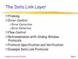
Data Link Layer Design Issues • Services Provided to the Network Layer • Framing • Error Control • Flow Control

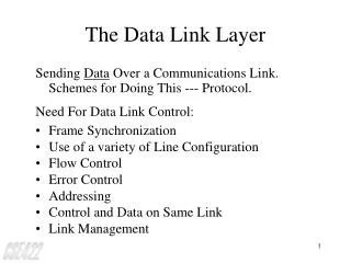
Data Link Layer Issues • Functions of the Data Link Layer • Provide service interface to the network layer • Dealing with transmission errors • Regulating data flow: Slow receivers not swamped by fast senders • To accomplish these goals, the data link layer encapsulates the packets into frames.

Functions of the Data Link Layer Relationship between packets and frames.

Services Provided to Network Layer (a) Virtual communication (model used). (b) Actual communication.

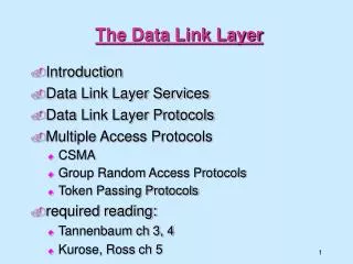
Services to the Network Layer • Three possible services offered by the data link layer: • Unacknowledged connectionless service: appropriate for channel with low error rate, real-time traffic, LAN • Acknowledged connectionless service: useful over unreliable channel such as wireless systems • Acknowledged connection-oriented service: used in routing

Services Provided to Network Layer Placement of the data link protocol.

Framing • To detect or correct errors in the raw bit stream from the physical layer, the data link layer breaks the bit stream up into discrete frames and computes the checksum for each frame. • Four methods can be used to mark the start and end of each frame: • Character count • Flag bytes with byte stuffing • Starting and ending flags, with bit stuffing • Physical layer coding violations

Framing A character stream. (a) Without errors. (b) With one error • Disadvantage: The count may be garbled. Rarely used.

Framing • Flag bytes with byte/character stuffing • Each frame start and end with special bytes – flag byte • If the flag byte occurs in the frame, stuff an extra escape byte (ESC). • Used in PPP (Point to Point Protocol) • Starting and ending flags, with bit stuffing • Each frame begins and ends with a special bit pattern 01111110 whenever the sender sees 5 consecutive 1s, it stuffs a 0. • Physical layer coding violations • Only applicable to networks in which the encoding on the physical medium contains some redundancy. • For example, a 1 bit is a high-low pair and a 0 bit is a low-high pair. High-high and low-low are used for delimiter.

Framing (a) A frame delimited by flag bytes. (b) Four examples of byte sequences before and after stuffing.

Framing Bit stuffing (a) The original data. (b) The data as they appear on the line. (c) The data as they are stored in receiver’s memory after destuffing.

Error and Flow Control • Error Control • Detect and/or correct errors • Ensure that all frame are eventually delivered in order  use acknowledgement, timer, and sequence number • Flow Control • Slow down the sender when the data is coming too fast for the receiver • Two approaches: • Feedback-based flow control – the receiver sends back permission to the sender. • Rate-based flow control – built-in mechanism that limits senders’ rate. Rarely used in the data link layer.

Error Detection and Correction • Error-correcting codes/forward error correction • include enough redundant information to enable the receiver to deduce the correct transmitted data. • Used in unreliable channel such as wireless links • Error-detecting codes • include only enough redundancy to allow the receiver to request a retransmission. • Used in reliable channel such as fiber

Error Correction Codes • N-bit codeword = m-bit data + r-bit check • The number of bit positions in which two codewords differ is called the Hamming distance. • Example: Hamming distance is 3. 10001001 xor 10110001 00111000 3 bit difference • If two codewords are a Hamming distance d apart, it will require d single-bit errors to convert one into the other.

Error Correction Codes • To detect d errors, we need a distance d+1 code (because there is no way to convert a valid codeword into another valid codeword with d changes.  The detail needs mathematical analysis). • Example: A simple error - detection code: (check bit) a parity bit is chosen so that the number of 1 bits in the codeword is even or odd. 000(0) - check bit 001 1 010 1 That is Hamming distance of parity bit code is 2 = d + 1  can detect d = 1 error

Error Correction Codes • To correct d errors, we need a distance 2d+1 code. (because d changes is not enough to recover the original valid codeword but only to convert to other valid codeword  The detail needs mathematical analysis). • Examples: Consider a code with four valid codewords: 0000000000, 0000011111, 1111100000, 1111111111 Hamming distance is 5. It can correct double errors. If 0000000111 is received, the receiver knows the original is 00000011111. But if a triple errors change 0000000000 to 0000000111, the error will not be corrected properly.

Error Correction Codes • Correct  round off to the nearest codeword. m data bits  2m legal messages = codewords • Examples: Consider a code with four valid codewords: 000000, 000111, 111000, 111111 differ by 3 011000, 101000, 110000, 111001, 111010, and 111100are six invalid code words a distance 1 from111000.  each valid codeword has n invalid codewords within hamming distance 1. To correct these n invalid codewords with 1 bit error, n + 1 bit patterns are required.

Error Correction Codes • Since there are a total of 2n bit patterns  (n + 1) x 2m≤ 2n  (m + r + 1) x 2m≤ 2m+r  m + r + 1 ≤ 2r • Given m, this puts a lower limit on the number of check bits needed to correct 1 error. m = 7  7 + r + 1 ≤ 2r 8 ≤ 2r - r  r = 4

Hamming Codes • Bits are numbered from the left . Checkbits are bits numbered powers of 2. {1,2,4,8,...}. Each checkbit forces the parity of some collection of bits, including itself, to be even or odd. • To see which check bits the data in position k contributes to, write k as a sum of powers of 2.

Constructing Hamming Codes The codeword is 00110010000. • Consider an ASCII code H (1001000). Use even parity: H 1001000 _ _ 1 _ 001 _ 000

Hamming Codes • When a codeword arrives, counter = 0. If a checkbit k does not have the correct parity, it adds k to the counter. • Supposed there is only one bit error. If counter = 0  no error If counter = 11  bit 11 in error. ASCII codeword H 1001000 0 0 1 1 001 0 000 G 1100001 1 0 1 1 100 1 001 If G is received as (0) 0 1 1 100 1 001, 1st bit is incorrect. If G is received as (1)(0){0} 1 100 1 001 1st and 2nd has errors.  3rd bit is incorrect.

Error-Correcting Codes Use of a Hamming code to correct burst errors.

Cyclic Redundancy Check • A major goal in designing error detection algorithms is to maximize the probability of detecting errors using only a small number of redundant bits. • In general, correcting is more expensive than detecting and re-transmitting. • Add k bits of redundant data to an n-bit message • want to use k << n to detect errors • e.g., k = 32 and n = 12,000 (1500 bytes) • Represent n-bit message as n-1 degree polynomial • e.g., MSG=10011010 as M(x) = x7 + x4 + x3 + x1 • Let k be the degree of some divisor polynomial • e.g., G(x) = x3 + x2 + 1

Cyclic Redundancy Check • CRC is a polynomial code. Frame 110001 represents x5 + x4 + x0 Polynomial arithmetic is performed modulo 2. 10011011 11001010 01010001  EX-OR result. • Sender & receiver agree upon a 'generator polynomial' G(x).

Cyclic Redundancy Check • Algorithm for computing the checksum • shift left r bits (append r zero bits to low order end of the frame), i.e., M(x)xr • divide the bit string corresponding to G(x) into (xr)M(x). • subtract (or add) remainder of M(x)xr / G(x) from M(x)xr using XOR,call the result T(x). Transmit T(x).

Cyclic Redundancy Check • Suppose that a transmission error E(x) has occured and T(x)+E(x) arrives instead of T(x). Received polynomial T(x) + E(x) = (T(x)+E(x))/G(x) = T(x)/G(x) + E(x)/G(x) = E(x)/G(x) • E(x) = 0 implies no errors • Divide (T(x) + E(x)) by G(x); remainder zero if: • E(x) was zero (no error), or • E(x) is exactly divisible by C(x)

CRC Example 11111001 ----------- 1101 /10011010000 <- Message 1101 ----- 1001 1101 ----- 1000 1101 ----- 1011 1101 ---- 1100 1101 ----- 1000 1101 ---- 101 <- Remainder • M(x)=10011010 • C(x)=1101 • k=3 • P(x) = 10011010 101

CRC Example 1100001010 -------------- 10011 /11010110110000 10011 ----- 10011 10011 ----- 10110 10011 ----- 10100 10011 ----- 1110 • M(x)=1101011011 • C(x)=10011 • k=4 • P(x) = 1101011011 1110

Error-Detecting Codes Calculation of the polynomial code checksum.

Selecting G(x) • All single-bit errors, as long as the xk and x0 terms have non-zero coefficients. • All double-bit errors, as long as G(x) contains a factor with at least three terms • Any odd number of errors, as long as G(x) contains the factor (x + 1) • Any ‘burst’ error (i.e., sequence of consecutive error bits) for which the length of the burst is less than k bits. • Most burst errors of larger than k bits can also be detected

Selecting G(x) • International standards for G(x): CRC-12 = x12+x11+x3+x2+x1+1 CRC-16 = x16+x15+x2+1  16 bit check sum.  catches all single, double,odd errors.  catches all burst errors of length < 16 • A simple shift register circuit can be constructed to compute and verify the checksums in hardware.

Elementary Data Link Protocols • An Unrestricted Simplex Protocol • connectionless • the sender continues sending frames with no acknowledge • the receiver has an infinite buffer. • A Simplex Stop-and-Wait Protocol • assume error free channel. • the sender sends frames only after getting an acknowledge • the receiver has finite buffer.

Elementary Data Link Protocols • A Simplex Protocol for a Noisy Channel connectionless • Positive Acknowledge and Retransmission (PAR) • if frames may be lost or acknowledged, then a time-out is required. • time-out must be long enough to account for the max. possible delay • need time-outs and sequence #'s. • Since only adjacent frames may conflict, we can use 2 sequence #'s 0 & 1.  sequence # only requires 1 bit.

Protocol Definitions Continued  Some definitions needed in the protocols to follow. These are located in the file protocol.h.

Protocol Definitions(ctd.) Some definitions needed in the protocols to follow. These are located in the file protocol.h.

Unrestricted Simplex Protocol

Simplex Stop-and-Wait Protocol

A Simplex Protocol for a Noisy Channel A positive acknowledgement with retransmission protocol. Continued 

A Simplex Protocol for a Noisy Channel (ctd.) A positive acknowledgement with retransmission protocol.

Sliding Window Protocols • In stop-and-wait protocols, latency at the sender is high  channel utilization (efficiency) is low. • Piggybacking is a technique of attaching a acknowledgement to a data frame. • In window-based Protocols, the sender's (receiver's) window is the range of sequence numbers which the sender (receiver) is allowed to send (receive) before blocking. • Pipelining means to increase the sender’s window size and transmit more than one frame before waiting for an acknowledge.

Sliding Window Protocols • Sliding Window Protocols • A One-Bit Sliding Window Protocol • A Protocol Using Go Back N • A Protocol Using Selective Repeat • Two approaches to deal with errors in pipelining: • Go Back N – Recovery by timeout-receiver discards all subsequent frames and sends no acknowledge. • Selective repeat – Special frame - receiver acknowledges with a special frame to start retransmit from missed frame.

Sliding Window Protocols A sliding window of size 1, with a 3-bit sequence number. (a) Initially. (b) After the first frame has been sent. (c) After the first frame has been received. (d) After the first acknowledgement has been received.

A One-Bit Sliding Window Protocol Continued 

A One-Bit Sliding Window Protocol (ctd.)

A One-Bit Sliding Window Protocol Two scenarios for protocol 4. (a) Normal case. (b) Abnormal case. The notation is (seq, ack, packet number). An asterisk indicates where a network layer accepts a packet.

A Protocol Using Go Back N • Receiver will only accept the next frame in the sequence. • Advantage: simple. • Disadvantage: Waste bandwidth if high error rate exists.

A Protocol Using Go Back N Pipelining and error recovery. Effect on an error when (a) Receiver’s window size is 1. (b) Receiver’s window size is large.

Sliding Window Protocol Using Go Back N Continued 

The Data Link Layer