Download
1 / 35
2.59k likes | 6.73k Vues
Chapter 6: Hydrographs. Previous Chapter estimation of long-term runoff was examined the present chapter examines in detail the short-term runoff phenomenon by the storm hydrograph or flood hydrograph or simply Hydrograph

E N D
Chapter 6: Hydrographs • Previous Chapter estimation of long-term runoff was examined • the present chapter examines in detail the short-term runoff phenomenon by the storm hydrograph or flood hydrograph or simply Hydrograph • The runoff measured at the stream-gauging station will give a typical hydrograph as shown in Fig. 6.1
The flood hydrograph is formed as a result of uniform rainfall of duration, Tr,. over a catchment. • The Hydrograph (Figure 6.1) has three characteristic regions: (i) the rising limb AB, joining point A, the starting point of the rising curve and point B, the point of inflection, (ii) the crest segment BCbetween the two points of inflection with a peak P in between, (iii) the falling limb or depletion curve CDstarting from the second point of inflection C.
Timing of the Hydrograph • tpk : the time to peak (Qp) from the starting point A, • lag time TL: the time interval from the centre of mass of rainfall to the centre of mass of hydrograph, • TB : the time base of the hydrograph • Factor Influencing the Hydrograph 1. Watershed Characteristics such as size, shape, slope, storage 2. Infiltration Characteristics soil and land use and cover 3. Climactic Factors • rainfall intensity and pattern • aerial distribution • duration • type (rainfall vs snowmelt) Generally, the climatic factors control the rising limb catchment characteristics determine the recession limb
6.3 COMPONENTS OF A HYDROGRAPH the essential components of a hydrograph are: (i) the rising limb, (ii) the crest segment, and (iii) the recession limb. crest Recession curve Concentration curve Rising limb Falling limb Inflection Point Q (m3/s) D.R. baseflow Time
Rising Limb • The rising limb of a hydrograph (concentration curve) represents the increase in discharge due to the gradual building up of storage in channels and over the catchment surface. • As the storm continues more and more flow from distant parts reach the basin outlet. At the same time the infiltration losses also decrease with time. Crest • The peak flow occurs when the runoff from various parts of the catchment at the same time contribute the maximum amount of flow at the basin outlet. • Generally for large catchments, the peak flow occurs after the end of rainfall, • the time interval from the centre of mass of rainfall to the peak being essentially controlled by basin and storm characteristics.
Recession Limb • It extends from the point of inflection at the end of the crest segment to the start of the natural groundwater flow • It represents the withdrawal of water from the storage built up in the basin during the earlier phases of the hydrograph. • The starting point of the recession limb (the point of inflection)represents the condition of maximum storage. • Since the depletion of storage takes place after the end of rainfall, the shape of this part of the hydrograph is independent of storm characteristics and depends entirely on the basin characteristics. • The storage of water in the basin exists as • surface storage, which includes both surface detention and channel storage, • interflow storage, and • groundwater storage, i.e. base-flow storage.
Barnes (1940) showed that the recession of a storage can be expressed as which Q0: the initial discharge and Qt :are discharges at a time interval of t days; K: is a recession constant of value less than unity. • Previous Equation can also be expressed in an alternative form of the exponential decay as where a =-In K, • The recession constant K; can be considered to be made up of three components to take care of the three types of storages as: K= Krs. Kri . Krb where Krs= recession constant for surface storage (0.05 to 0.20), Kri= recession constant for interflow (0.50 to 0.85) and Krb= recession constant for base flow (0.85 to 0.99) Example 6.1
6.4 Base Flow Separation • The surface hydrograph is obtained from the total storm hydrograph by separating the quick-response flow from the slow response runoff. • The base flow is to be deducted from the total storm hydrograph to obtain the surface flow hydrograph in three methods
Method I: Straight line method • Draw a horizontal line from start of runoff to intersection with recession limb (Point A). • Extend from time of peak to intersect with recession limb using a lag time, N. N =0.83 A0.2 Where: A = the drainage area in Km2 and N = days where Point B can be located and determine the end of the direct runoff .
Q N B A C time Method II: In this method the base flow curve existing prior to the beginning of the surface runoff is extended till it intersects the ordinate drawn at the peak (point C in Fig, 6.5). This point is joined to point B by a straight line. Segment AC and CB separate the base flow and surface runoff. This is probably the most widely used base-flow separation procedure.
N Q t Method III In this method the base flow recession curve after the depletion of the flood water is extended backwards till it intersects the ordinate at the point of inflection (line EF in Fig. 6.5), Points A and F are joined by an arbitrary smooth curve. This method of base-flow separation is realistic in situations where the groundwater contributions are significant and reach the stream quickly. The selection of anyone of the three methods depends upon the local practice and successful predictions achieved in the past. The surface runoff hydrograph obtained after the base-flow separation is also known as direct runoff hydrograph (DRH). Method V
Rainfall Excess 6.5 EFFECTIVE RAINFALL • Figure 6.6. show, the hyetograph of a storm. The initial loss and infiltration losses are subtracted from it. The resulting hyetograph is known' as effective rainfall hyetograph (ERH). It is also known as hyetograph of rainfall excess or supra rainfall. • Both DRH and ERH represent the same Total quantity but in different units • ERH is usually in cm/h against time • The area multiplied by the catchment Area gives the total volume of the direct runoff ( total area of DRH)
6.6 UNIT HYDROGRAPH • A large number of methods are proposed to solve this problem and of them probably the most popular and widely used method is the unit-hydrograph method. • A unit hydrograph is defined as the hydrograph of direct runoff resulting from one unit depth (1 cm) of rainfall excess occurring uniformly over the basin and at a uniform rate for a specified duration (D hours). • The term unit here refers to a unit depth of rainfall excess which is usually taken as 1 cm. • The duration, being a very important characteristic, is used as indication to a specific unit hydro graph. Thus one has a 6-h unit hydrograph, 12-h unit hydrograph, etc. and in general a D-h unit hydrograph applicable to a given catchment.
The definition of a unit hydrograph implies the following: • It relates only the direct runoff to the rainfall excess. Hence the volume of water contained in the unit hydrograph must be equal to the rainfall excess. As 1 cm depth of rainfall excess is considered the area of the unit hydrograph is equal to a volume given by 1cm over the catchment. • The rainfall is considered to have an average intensity of excess rainfall (ER) of l/D cm/h for the duration D-h of the storm. • The distribution of the storm is considered to be uniform all over the catchment.
Fig 6.9 shows a typical 6-h unit hydrograph. Here the duration of the rainfall excess is 6 h Area under the unit hydrograph = 12.92 X 10⁶ m3
Two basic assumptions constitute the foundations for the unit-hydrograph theory: • the time invariance and • the linear response. Time Invariance This first basic assumption is that the direct-runoff response to a given effective rainfall in a catchment is time-invariant. This implies that the DRH for a given ER in a catchment is always the same irrespective of when it occurs.
Linear Response • The direct-runoff response to the rainfall excess is assumed to be linear. This is the most important assumption of the unit-hydrograph theory. • Linear response means that if an input xI (t) causes an output yI(t) and an input .x2 (t) causes an output y2 (t), then an input xl(t) +x2 (t) gives an output y1 (t) +y2(t). • Consequently, if x2 (t) = r XI(t), then yz (t) = r yI(t). • Thus if the rainfall excess in a duration D is r times the unit depth, the resulting DRH will have ordinates bearing ratio r to those of the corresponding D-h unit hydrograph.
Since the area of the resulting DRH should increase by the ratio r, the base of the DRH will be the same as that of the unit hydrograph. If two rainfall excess of D-h duration each occur consecutively, their combined effect is obtained by superposing the respective DRHs with due care being taken to account for the proper sequence of events. (The method of superposition )
The desired ordinates of the DRH are obtained by multiplying the ordinates of the unit hydrograph by a factor of 3.5 as in Table 6.3. Note that the time base of DRH is not changed and remains the same as that of the unit hydrograph.
Application of U-Hydrograph D-h U-hydrograph and storm hyetograph are available ERH is obtained by deducting the losses ERH is divided by M blocks of D-h duration Rainfall excesses is operated upon unit hydrograph successively to get different DHR curves
6.7Derivation of Unit Hydrographs • The area under each DRH is evaluated and the volume of the direct runoff obtained is divided by the catchment area to obtain the depth of ER. • The ordinates of the various DHRs are divided by the respective ER values to obtain the ordinates of the unit hydrograph.
Solution of Example 6.7 • However, N =2.91 days is adopted for convenience. • A straight line joining A and B is taken as the divide line for base-flow separation. • The ordinates of DRH are obtained by Subtracting the base flow from the ordinates of the storm hydrograph.
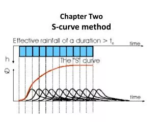
6.8 Unit Hydrographs of Different Duration • Unit hydrograph are derived from simple isolated storms and if the duration of the various storms do not differ two much (20% D) >>>> make the average duration of D h. • In practice the unit hydrographs of different duration are needed (nD). • Two methods are available • Method of Superposition • the S-Curve
6.8 Unit Hydrographs of Different Duration • Unit hydrograph are derived from simple isolated storms and if the duration of the various storms do not differ two much (20% D) >>>> make the average duration of D h. • In practice the unit hydrographs of different duration are needed (nD). • Two methods are available • Method of Superposition • the S-Curve
Method of Superposition • D-H unit duration is available and it is needed to make UH of nDH, where n is and integer • Superposing n UH with each graph separated from the previous one by D h.
HW6 • 6.4 • 6.7 • 6.9 • 6.13 • 6.19


![Hydrographs [Date] Today I will: - Be able to construct and understand flood hydrographs](https://cdn3.slideserve.com/5580541/hydrographs-date-today-i-will-be-able-to-construct-and-understand-flood-hydrographs-dt.jpg)