Download
1 / 85
920 likes | 1.76k Vues
Government Intervention in Market Failure. Chapter 3. © 2004 Thomson Learning/South-Western. Topics in Chapter 3. Should the Government Intervene? Are there private solutions that will work? Types of Government Intervention – general introduction The “optimal” level of environmental quality

E N D
Government Intervention in Market Failure Chapter 3 © 2004 Thomson Learning/South-Western
Topics in Chapter 3 • Should the Government Intervene? Are there private solutions that will work? • Types of Government Intervention – general introduction • The “optimal” level of environmental quality • Government intervention: Command and Control policies • Government intervention: Economic incentives
Should the Government Intervene? Pigouvian Taxes • A.C. Pigou (1938) argued that an externality cannot be mitigated by contractual negotiation between the affected parties. • Pigou argued that direct coercion by the government or judicious use of taxes should be used against the offending party. • These taxes are referred to as Pigouvian taxes.
Pigouvian Taxes • The basic principle behind the use of externality taxes is that the tax eliminates the divergence between the Marginal Private Cost (MPC) and the Marginal Social Cost (MSC). • Q1 represents the market equilibrium (where MPC=MPB), and • Q* represents the optimal level of output (where MSC=MSB).
An Externality Tax on Output MSC = MPC + MDpollution $ a MPC1 b Demand Quantity of steel Q1 Q*
Pigouvian Taxes • An externalities tax equal to the divergence between MPC and MSC would raise the steel firms’ private costs. • The tax would shift the MPC curve by an amount equal to the distance from a to b in Figure 3.1. • The market would arrive at an optimal equilibrium of Q*. • This is known as internalizing an externality. • More precisely, the tax should be placed on the externality itself (the amount of pollution emissions) rather than on output (amount of steel).
Coase Theorem • Ronald Coase (1960) argued that not only is a tax unnecessary, it is often undesirable. • Coase argued: • The market will automatically generate the optimal level of the externality. • This optimal level of the externality will be generated regardless of the initial allocation of property rights.
Coase Theorem • One example to illustrate his theory is based on the interaction of a cattle rancher and a crop farmer. • Cattle occasionally leave rancher’s property and damage farmer’s crop. • Coase argued that the farmer and rancher will reach an agreement that will make them both better off. • Either the rancher will accept payment to reduce the size of the herd or farmer will accept payment to cover cost of crops lost. • And this will happen without government intervention.
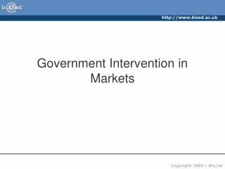
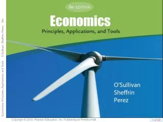
Another example: Dorm room stereos and studying $ MC loudness to you D = MB loudness to partier Q0 Q* QL Loudness
Dorm room stereos and studying • If property rights belong to partier, where is initial noise level? QL • But there are gains from trade until move back to Q* • If property rights belong to partier, where is initial noise level? Q0 • Again, gains from trade until get to Q* • Gains to be split between two parties are denoted “A” and “B” in diagram
Another example: Dorm room stereos and studying $ D = MB loudness to partier MC loudness to you A B Q0 Q* QL Loudness
Coase Theorem • If there are no transaction costs and property rights are well defined, then voluntary transactions will eliminate any distortions in resource allocation stemming from an externality and the outcome is independent of the property rights • This version of the “theorem” is from Baumol and Oates text “The Theory of Environmental Policy.” • Emphasizes private behavior and importance of transaction costs
Coase Theorem • What happens if impose a Pigouvian tax on the generator of the externality, would this result in an efficient outcome? • Set a tax equal to marginal damage at the optimal to shift the demand for loudness • After the tax, are there still gains from trade? • Would tax be a good idea? • This is basis for Coase’s argument that government intervention could make things worse
Coase with a tax per unit of Loudness $ MC loudness to you D = MB loudness to partier - tax D = MB loudness to partier tax Q0 QN Q* QL Loudness
Criticisms: Coase Theorem • Two important assumptions: transactions costs are insignificant and property rights well defined. • Transactions costs are costs associated with arriving at an agreement (the costs of negotiation). • These may be small for a 2 party agreement but would be very large for an externality such as sulfur dioxide emissions across North America.
Coase Theorem • The number of participants makes transactions costs important. • One way to reduce transactions costs is to appoint an agent who acts in behalf of a large number of people. • The use of agents is associated with its own problems: • Free riders – don’t share in cost, but share benefits. • Often it is difficult for individuals to identify the agent that will best represent their view point.
Coase Theorem • Another problem associated with the Coase example can occur when the allocation of property rights would signal entry and exit in response to those rights. • If ranchers have the right to let their cattle roam without worrying about paying damages, then there can be an increase in the number of ranchers, and more damage.
Bottom Line on Coase arguments • Probably are cases where private negotiations can be effective • In those cases, government should stay out • But, probably plenty of cases where transaction costs and other issues lead to need for intervention
Types of Government Intervention • There are five broad classes of government intervention: • Moral suasion • Direct production of environmental quality • Pollution prevention • Command and control regulations • Economic incentives • Each of these represents a different philosophy toward the role of government in society.
Moral Suasion • This term is used to describe government attempts to influence behavior without actually stipulating any rules. • Effectiveness depends upon the extent to which individuals believe it is in their collective interest to do so. • Successful programs include Woodsy Owl’s “Give a hoot, don’t pollute” and Smokey Bear’s “Only you can prevent forest fires.”
Direct Production of Environmental Quality • Includes • reforestation, • breaching of dams, • stocking of fish, • creation of wetlands, • treatment of sewage, and • toxic waste site cleanup. • These are sometimes ameliorative actions.
Pollution Prevention • Designed to address market failure of imperfect information, in some cases there may be technologies that could be developed that save firm’s money and improve environment • Basic premise is that combined efforts of government agencies, national laboratories, university and private firms can lead to development of innovative and beneficial technologies. • These programs emphasize being proactive in reducing pollution, encourage R&D and adoption of “green technologies” .
Command and Control Regulation • These place constraints on the behavior of households and firms. • Constraints generally take the form of limits on inputs or outputs in the consumption or production process. • Examples include: • Requiring sulfur-removing scrubbers on the smokestacks of coal-burning utilities. • Prohibitions against dumping of toxic substances.
Economic Incentives • Economic incentives make self interest coincide with social interest. • Examples include: • Pollution taxes • Pollution subsidies • Marketable pollution permits • Deposit-refund systems • Performance bonds • Liability systems
Choosing the Correct Level of Environmental Quality • Zero pollution is not possible/desirable for two reasons: • The reduction of pollution will have opportunity costs. • The Law of Mass Balance makes a choice of zero physically impossible. • The Law of Mass Balance states that the mass of outputs of any activity are equal to the mass of inputs. • Any consumption or production activity must produce waste.
Choosing the Correct Level of Environmental Quality Definitions first: • Stock pollutants: pollutants for which environment has little ability to absorb: non biodegradable bottles, heavy metals, toxics • Fund pollutants: environment has some ability to absorb, pollutant doesn’t accumulate indefinitely; organic pollutants, CO2 absorbed by plants, etc. • Focus now on Fund Pollutants
Choosing the Correct Level of Environmental Quality • The desired level of pollution will be a function of the social costs associated with pollution. • The first of these is the damage that pollution creates by degrading the physical, natural, and social environment. • The second is the cost of reducing pollution and includes the opportunity costs of resources used to reduce pollution and the value of foregone outputs.
The Marginal Damage Function • The marginal damage function represents the damages that pollution generates by degrading the environment. • Even if these impacts are not quantifiable, the marginal damage function is useful for thinking about the relationship between environmental change and social welfare.
Marginal Damage Function • The marginal damage function specifies the damages associated with an additional unit of pollution. • The total damages generated by a particular level of pollution is represented by the area under the marginal damage function.
Marginal Damage Function • The increasing slope of the marginal damage function indicates how damage changes with each additional unit of pollution. • An upward sloping marginal damage function indicates that as the level of pollution becomes larger, the damages associated with the marginal unit of pollution become larger.
Marginal Abatement Cost Function • Abatement Costs are those costs associated with reducing pollution to a lower level so that there are fewer damages. • Abatement costs include: • Labor • Capital • Energy needed to lessen emissions • Opportunity costs from reducing levels of production or consumption.
Marginal Abatement Cost Function • The marginal abatement cost function represents the costs of reducing pollution by one more unit. • In the following figure, Eu represents the level of pollution that would be generated in absence of any government intervention. • As pollution is reduced below Eu, the marginal abatement cost increases.
Marginal Abatement Cost Function • Marginal abatement costs rise as cheaper options for reducing pollution are exhausted and more expensive steps must be taken. • The decreasing slope indicates that the costs of reducing pollution increases at an increasing rate. • A high vertical intercept indicates that the cost of eliminating the last few units of pollutants would be extremely high.
The Optimal Level of Pollution • Optimal level of pollution minimizes the total social costs of pollution (the sum of total abatement costs and total damages). • This level occurs at the point where marginal abatement costs are equal to marginal damages.
The Optimal Level of Pollution • If the level of emissions is less than E1, then the marginal abatement costs are greater than the marginal damages that the unit of pollution would have caused. • It doesn’t make sense to reduce pollution. • If the level of emissions are greater than E1, then the marginal damages are greater than the marginal abatement costs associated with reducing pollution by one unit. • Society is better off eliminating that unit of pollution.
Social Costs When Pollution Level is Greater than Optimal • The optimal level of pollution is E1. • The actual level of pollution is E2. • Total costs associated with pollution have been increased by the area of triangle abc. • This represents marginal damages greater than marginal abatement costs for the range of pollution emissions between E1 and E2.
Social Costs When Pollution Level is Less than Optimal • The optimal level of pollution is E1. • The actual level of pollution is E3. • Total costs associated with pollution have been increased by the area of triangle ade. • This represents marginal abatement costs greater than marginal damage for the range of pollution emissions between E1 and E3.
Optimal Level of Pollution, an alternative graphical representation damages, costs, $ MAC MDF = MB abatement A1 Abatement
Optimal Level of Pollution, an alternative approach • Plot functions against “abatement” instead of pollution • Abatement is the amount of pollution reduced • These are analagous approaches, just sometimes more convenient to think in terms of abatement vs. pollution • Answers are the same.
Optimal Level of Pollution, two approaches on one graph = MB emissions = MB abatement abatement
Optimal pollution (abatement) levels and costs of control • Two goals of environmental policy • Get the optimal amount of pollution (abatement) – just discussed • Achieve that level at the lowest possible cost • Goals are actually inter related, but helpful to think about them in two steps, once have identified optimal amount of pollution, how to achieve it at least cost
Optimal pollution (abatement) levels and costs of control • Suppose optimal to control (abate) 100 units of pollution that are generated by two firms • How much control should each firm undertake to minimize total costs • Plot abatement levels by the two firms against each other with a total of 100 units of abatement • Cost of control is at a minimum when the marginal abatement costs are equal
Least cost allocation of abatement between two sources (firms) damages, costs, $ MAC1 MAC2 b a 0 10 20 30 40 50 60 70 80 90 100 100 90 80 70 60 50 40 30 20 10 0 Abatement firm 1 Abatement firm 2