Download

1 / 19
190 likes | 210 Vues
This paper discusses efficient IP routing lookup algorithms for high performance packet forwarding in rapidly growing internet networks. It compares binary search-based methods with trie-based methods and introduces the concept of mutating binary search. The implementation and possible variations of the algorithms are also explored.

E N D
IP Routing Lookups Scalable High Speed IP Routing Lookups. Based on a paper by: Marcel Waldvogel, George Vaghese, Jon Turner, Bernhard Plattner.
Background and Motivation • Rapidly growing Internet increases demands for high performance routing. • Routing table lookup for a destination address is one of the key components of packet forwarding. • Given IP address, find out the output link that is the best choice to reach this IP. • Hierarchial IP address structure. • BMP – Best matching prefix problem.
The Address Lookup Problem • Address in a packet is compared to the stored prefixes starting from the left most bit. • The longest prefix found is the desired match. • The packet is forwarded to the specific next hop. • Next hop field changes – topology, traffic. • Set of prefixes changes rarely – inserting/removing network or host.
Address lookup using Tries 1 0 0 1 0 Existing prefixes: 000, 001, 010, 011, 100, 101, 11, 111 1 • Prefixes stored in a binary trie • Black nodes denote terminal nodes for prefixes. • Remember the most recent black node. • The search ends either in leaf or because of no matching branch to follow. • Time Complexity W (= 32 for IPv4 and 128 for IPv6) memory accesses. 1 1 0 1 0 0 1
Liner Search of Hash Tables • Organize prefixes into the hash tables by length. • Start searching from the longest prefix size. • W hash function computations in the worst case. W = maximal prefix length, 32 for IPv4.
Binary Search of Hash Tables.(Basic Scheme) • Organize prefixes into the hash tables by length. • Introduce markers. • Remember the last found BMP to avoid backtracking. • log2w hash function computations.
Binary Search of Hash Tables. Binary search Hash tables Hash tables with markers Prefix length 0 1 P1=0 P1=00 11 00 2 P3=111 111 3 - Prefix 00 - Marker 11
Binary Search of Hash Tables. (Code) Binary_Search(D) // Search for address D Initialize search range R to cover the whole array L; InitializeBMP found so far to NULL; While R is not empty { Let i correspond to the middle level in range R; Extract the first L[i].length() bits of D into D’; M = Search(D’,L[i].hash); // search hash for D’ if (M == NULL) R = Upper half of R; // Not found else if (M is a prefix and not a marker) { BMP = M.bmp; break;} else { // M is a pure marker or a marker and a prefix BMP = M.bmp; // update the best matching prefix so far R = lower half of R; } End;
Mutating Binary Search • Every match in the binary search with some marker X • means that we need only search among the set of prefixes for which X is a prefix. • BS mutates (changes) the levels on which it searches dynamically • (in a way that always reduces the level to be searched) as it gets more match information. • Average number of memory lookups is 2 for IPv4 (32 bit) Root New Trie on failure m = median length among all prefix lengths in trie X New Trie on match (first m bits of Prefix = X)
Mutating Binary Search (example:) Prefix length Mutating search trees Hash Tables 16 E: …, Tree2 17 18 19 F: ...111, Tree3 H: ...101, Tree4 20 J: …1010, End 21 G: …11100, End H: ...101, Tree4 22 23 24 Node_Name: Prefix(… stands for E), Tree to use from now on Hash entry structure:
Mutating Binary Search:Advantages / Disadvantages • Advantages: • Faster average lookup time. • Disadvantages: • Increased new prefix insertion time. • Increased storage requirements for optimal binary search trees family.
Mutating Binary Search:How to reduce the storage needed? • On match we use the new tree • On miss we use only the upper part of the current tree • We never use more then a single rope like branch from any specific tree. • So we can store ropes instead of binary trees
Ropes of a sub tree – the sequence of levels which binary search will follow on repeated failures. Example: Prefix length Mutating search trees Hash Tables 16 E: …, Tree2 17 18 19 F: ...111, Tree3 H: ...101, Tree4 20 J: …1010, End 21 G: …11100, End H: ...101, Tree4 22 23 24
Rope Variation of Mutating Binary SearchSearch for address D: Rope Search(D) { Rdefault search sequence BMPNULL While R is not empty { i first pointer found in R D’first L[i].length() bits of D M Search(D’,L[i].hash) // search hash for D’ if (M != NULL) { BMP M.bmp //update the best matching prefix so far R M.rope //get the new Rope, possibly empty } } }
Possible variations • Arrays usage instead of hash tables for the initial prefix lookup. • Space time tradeoff : • wo prefix length for which array is used (wo=16) • 2Wo space used (216) • Hardware implementations. • Rope search algorithm is simple • Can be pipelined
Mutating Binary Search:Implementation: • Precomputations – building the rope search data structure optimized for a given prefix set. • Insertions/deletions result in performance degradation
Conclusions: • Simple Binary search algorithm reduce number of memory accesses from W to log 2W. Where w = number of bits in the IP address. (5 = log 232 hash computations for IPv4) • Mutating Binary search algorithm further reduce the average case hash computations number to 2. • The DS initialization takes O(sum of prefix lengths)
Practical Measurements: • Practical measurements made on 200 MHz Pentium Pro, C using compiler max. optimizations on table with 33,000 entries • about 80ns for IPv4 • about 150-200ns for IPv6
Generalized Level Compressed Tries. • Definition – Tries with n levels compressed into the hash tables. • Time complexity optimization problem under memory constrains. • To be presented the next lecture.