Download
1 / 42
430 likes | 533 Vues
Matched Filter Search for Ionized Bubbles in 21-cm Maps. Kanan K. Datta. Dept. of Astronomy Stockholm University. Oskar Klein Centre. Collaborators. Somnath Bharadwaj Tirthankar Roy Choudhury Suman Majumdar. 21 cm observations of the reionization : Major Approaches.

E N D
Matched Filter Search for Ionized Bubbles in 21-cm Maps Kanan K. Datta Dept. of Astronomy Stockholm University Oskar Klein Centre
Collaborators • Somnath Bharadwaj • TirthankarRoy Choudhury • SumanMajumdar
21 cm observations of the reionization : Major Approaches • Global evolution of average redshifted 21 cm differential brightness temperature with redshift. (Ravi Subramanian’s talk) • The rms, skewness measurement as a function of redshift. (GarreltMellema’s talk) • Measuring HI power spectrum. (AbhikGhosh, Somnath Bharadwaj, Stuart Wyithe’s talk) • Cross – Correlation (Brigs, T. GuhaSarkar’s talk) 5) Detecting Individual Ionized Bubbles
Ionized bubbles HI
Can we detect individual ionized bubbles in 21-cm observations?
Motivation for Individual Bubble detection Direct probe of reionization. Interpretation is easier. IGM properties (HI fraction surrounding the HII regions) Source properties (age, photon emission rate ) This will compliment the study through power spectrum measurements
A Visibility based method • Direct measured quantity is Visibility • Noise in the image is correlated, where as in visibility it is uncorrelated. Advantages over the image base method
A Visibility based method • To optimally combine the signal from an ionized bubble of radius R_b at redshift z_c we introduce anestimator
A Visibility based method • To optimally combine the signal from an ionized bubble of radius R_b at redshift z_c we introduce anestimator Total Observed visibility
A Visibility based method • To optimally combine the signal from an ionized bubble of radius R_b at redshift z_c we introduce anestimator Filter
A Visibility based method • To optimally combine the signal from an ionized bubble of radius R_b at redshift z_c we introduce anestimator Summation over all baselines and frequency channels
A Visibility based method • To optimally combine the signal from an ionized bubble of radius R_b at redshift z_c we introduce anestimator Analytically the mean also can be calculated using
A Visibility based method • To optimally combine the signal from an ionized bubble of radius R_b at redshift z_c we introduce anestimator Analytically the mean also can be calculated using Baseline Distribution function
Simulating Signal • Simulate dark matter distribution at redshift 6 • Grid size=2 Mpc, Box size=256 Mpc (GMRT), 512 Mpc (MWA) Dark Matter map
Simulating Signal • Simulate dark matter distribution at redshift 6 • Grid size=2 Mpc, Box size=256 Mpc (GMRT), 512 Mpc (MWA) • Assume HI traces Dark matter with bias 1 HI map
Simulating Signal • Simulate dark matter distribution at redshift 6 • Grid size=2 Mpc, Box size=256 Mpc (GMRT), 512 Mpc (MWA) • Assume HI traces Dark matter with bias 1 • We put spherical ionized bubbles by hand with one at the centre.
Simulating Signal • Simulate dark matter distribution at redshift 6 • Grid size=2 Mpc, Box size=256 Mpc (GMRT), 512 Mpc (MWA) • Assume HI traces Dark matter with bias 1 • We put spherical ionized bubbles by hand with one at the centre.
Simulating Signal • Simulate dark matter distribution at redshift 6 • Grid size=2 Mpc, Box size=256 Mpc (GMRT), 512 Mpc (MWA) • Assume HI traces Dark matter with bias 1 • We put spherical ionized bubbles by hand with one at the centre.
Simulating Signal • Simulate dark matter distribution at redshift 6 • Grid size=2 Mpc, Box size=256 Mpc (GMRT), 512 Mpc (MWA) • Assume HI traces Dark matter with bias 1 • We put spherical ionized bubbles by hand with one at the centre.
Simulated maps SB PR2 PR1
Simulating visibilities Effect of the HI fluctuations
Matched Filter The signal to noise ratio (SNR) is maximum if we use the filter exactly matched with the signal from the bubble that we are trying to detect ie.,
Matched Filter The signal to noise ratio (SNR) is maximum if we use the filter exactly matched with the signal from the bubble that we are trying to detect ie., To remove the foreground contribution we modifythe filter as, The filter subtracts out any frequency independent component from the frequency range
Results • Restriction on bubble detection: SB Detection of bubbles of radius >8 Mpc for GMRT is possible. HI fluctuations will affect Small bubble detection (<8 Mpc).
Bubble detection in Patchy reionization PR1 We get almost similar results for PR1 scenario.
Bubble detection in Patchy reionization PR1 We get almost similar results for PR1 scenario. In the PR2 scenario HI fluctuations will dominate over the bubble signal.
Size determination of ionized bubbles In reality bubble size and position not known. We have to find out size and positions (4 unknown parameters) We expect signal to noise ratio (SNR) to peak when the filter is exactly matched to the signal. We propose this can be used to measure bubble size.
SNR Filter Bubble
SNR !PEAK ! Filter Bubble
Credit: Suman Majumdar SNR Filter Bubble
Size determination We calculate the SNR for the filters for various sizes and find out peak SNR and calculate bubble size. With 1000 h of observations , SNR ~ 3 Datta, Majumdar, Bharadwaj, Choudhury, MNRAS,2008
Size determination is not limited by the HI fluctuations but limited by the resolution of the experiments This can be done more accurately for larger bubbles. 1000 hrs, SNR~ 9
SNR Bubble Filter
SNR !PEAK ! Filter Bubble
SNR Credit: Suman Majumdar Bubble Filter
Searching bubbles (Position determination) The bubble is placed at the center of the field of view (FoV) We move the center of the filter to different positions and search for a peak in the SNR. Datta, Majumdar, Bharadwaj, Choudhury, MNRAS,2008
Scaling Relations Source properties Reionization history Background Cosmology Instrument
ER LR Optimal Redshift We find that redshift range 7-9.2 and 8.8-10.8 are the most appropriate for the GMRT and the MWA respectively. A 3 sigma detection is possible with the GMRT for bubbles > 50 Mpc or >30 Mpc for 1000 hrs of integration time for ER or LR models. The same figure is >40 Mpc and >30 Mpc for the MWA. Datta, Bharadwaj, Choudhury, MNRAS, 2009
Conclusions • We developed a technique for detecting individual ionized bubbles in 21-cm maps. The technique maximizes the SNR and subtracts out foregrounds. • A 3 sigma detection is possible with instruments like GMRT, LOFAR, MWA for bubbles > 50 Mpc or >30 Mpc for ~1000 hrs of integration time for ER or LR models. • Bubble size can be determined which will give crucial information about reionizing source properties • Blind search for bubbles is, in principle possible. • Detailed study with simulated signal, foregrounds, noise etc needs to be done.