Download
1 / 16
160 likes | 276 Vues
Power Analysis. Many of you have seen OCC’s First specify test size a, s 2 , m in a CRD Compute : Compute. Power Analysis. Compute a summary measure of H a : OCC curves will depend on a , and the numerator and denominator df. Power Analysis. Select the appropriate OCC curve

E N D
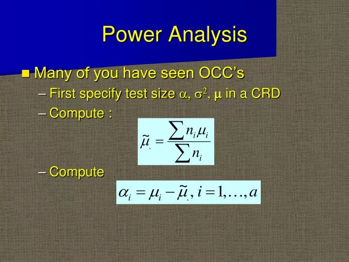
Power Analysis • Many of you have seen OCC’s • First specify test sizea, s2, min a CRD • Compute : • Compute
Power Analysis • Compute a summary measure of Ha: • OCC curves will depend on a, and the numerator and denominator df
Power Analysis • Select the appropriate OCC curve • Find where vertical line drawn fromfon horizontal axis intersects appropriate OCC • Readbon vertical axis; compute1-b
Power Analysis • OCC’s can be used for sample size analysis, but they are awkward • The curves are computed from the distribution of the F statistic under HA
Derivation of OCC’s • Recall that
Derivation of OCC’s • Regardless of the true state of nature, where
Derivation of OCC’s • A non-central c2 rv is often introduced as a sum of independent squared N(li,s2) rv’s; its noncentrality parameter would be: • In our case, the normal components are not independent.
Derivation of OCC’s • We say that F has a noncentral F distribution with noncentrality parameter d2 • A non-central F rv is based on a ratio of independent non-central c2 and central c2 rv’s
Derivation of OCC’s • For the balanced case, we have:
Computer Code • SAS example • R code S02<-rep(seq(1,5),rep(15,5)) n<-rep(seq(2,16),5) ncvec<-n*s02
Computer Code Power<-1-pf(qf(.95,a-1,n*a-a),a-1,n*a-a,ncvec) Contour(seq(2,16),seq(1,5),matrix(power,ncol=5),xlab=“Sample Size”,ylab=“Effect”)
Power Analysis for Contrasts • Magnitude of contrasts under HA is easy for experimenters to articulate (Yandell, Edwards) • We consider one df contrasts only (Yandell focuses on specific cases; our treatment will be more general)
Power Analysis for Contrasts • We will test Ho:L-Lo=0 vs. HA:L-Lo≠0 • Typically, Lo=0 • Regardless of the true state of nature,
Power Analysis for Contrasts • For the balanced case,
Power Analysis for Contrasts • To adapt the SAS program to contrasts, note that the coefficient of n in the noncentrality parameter has changed • Loop on L (not s02) and calculate s02 in the loop • This ensures that L is output rather than s02 • Remember to change numerator df