Download
1 / 33
340 likes | 512 Vues
Interactive Non-Photorealistic Rendering of Technical Illustrations. Daniel Weiskopf VIS Group, University of Stuttgart. Introduction. realistic rendering. non-photorealistic. Introduction. Photorealistic rendering Resemble the output of a photographic camera

E N D
Interactive Non-Photorealistic Renderingof Technical Illustrations Daniel WeiskopfVIS Group, University of Stuttgart
Introduction realistic rendering non-photorealistic
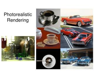
Introduction • Photorealistic rendering • Resemble the output of a photographic camera • Non-photorealistic rendering (NPR) • Convey meaning and shape • Emphasize important parts • Mimic artistic rendering
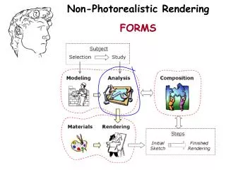
Introduction • Typical drawing styles for NPR • Pen-and-ink illustration • Stipple rendering • Tone shading • Cartoon rendering • Further reading on NPR: • SIGGRAPH 1999 Course #17: Non-Photorealistic Rendering • Gooch & Gooch: Non-Photorealistic Rendering [2001] • Strothotte & Schlechtweg: Non-Photorealistic Computer Graphics [2002]
Introduction • Focus of this talk • Technical illustrations • Tone shading: cool / warm shading • Semi-transparent rendering
Tone Shading • Cool / warm shading [Gooch et al. 1998] • Tone shading for technical illustrations • Lighting model: • Uses luminance and hue • Indicates surface orientation
N H L V Tone Shading • Standard Blinn-Phong model • Positive term max(0, LN) • L light vector • N normal vector • V viewing vector • H halfway vector
Tone Shading • Cool / warm shading of a matte object • Dot product LN between normal vector and light vector • LN can be negative: LN [-1,1] • Specular highlights like in Blinn-Phong model
Tone Shading • Mixture of yellow and the object’s color kd : • Mixture of blue and the object’s color kd : yellow user-specified diffuse object color blue user-specified diffuse object color
Implementation on Standard Hardware • Gouraud shading • Approximation via two light sources: • Light along direction L with intensity (kwarm – kcool)/2 • Light along direction -L with intensity (kcool – kwarm)/2 • Ambient term with intensity (kcool + kwarm)/2 • Object color has to be white • Problems: • No specular highlights (only in two-pass rendering) • Change of material parameters needs change of light color • Two light sources needed • Negative intensities for the light sources
Cool / Warm Shading via Vertex Programs • Gouraud shading • Implements cool / warm shading on per-vertex basis • Includes specular highlights • Computation in flexible vertex programs
Cool / Warm Shading via Vertex Programs • Only fragments of the vertex program code • Already done: • Transformation of vertex into eye and clip coordinates • Transformation of normal vector into eye coordinates • Computation of halfway vector • Input: • Diffuse object color as primary color • Parameters for cool / warm model • Parameters for specular highlights • Color and direction of light
Cool / Warm Shading via Vertex Programs • First part: computation of geometric components for lighting ... # c[0] = L: direction of light # c[1].x = m: shininess for highlight # R0 = N: normal vector in eye coords # R1 = H: halfway vector in eye coords DP3 R2.x,c[0],R0; # L*N DP3 R2.y,R1,R0; # H*N MOV R2.z,c[1].x; # shininess for highlight LIT R3,R2; # R3=weights for Blinn-Phong ... # model
# R6 = (k_d*beta + k_yellow) = k_warm Cool / Warm Shading via Vertex Programs • Parameters for cool / warm shading • Analogous: # v[COL0] = k_d : diffuse material color # c[2] = (alpha,beta,0,0): cool/warm params # c[3] = k_blue: blue tone MOV R4,c[2]; MAD R5,v[COL0],R4.x,c[3]; #(k_d*alpha + k_blue) # = k_cool
# c[4] = (1,0.5,0,0) # R2.x = L*N ADD R7,R2.x,c[4].x; # L*N + 1 MUL R8,R7,c[4].y; # (L*N + 1)/2 ADD R9,-R8,c[4].x; # 1 - (L*N + 1)/2 # R5 = k_cool # R6 = k_warm MUL R10,R5,R9; # warm part MAD R10,R6,R8,R10; # add cool part Cool / Warm Shading via Vertex Programs • Geometric coefficients for cool / warm shading • Cool / warm shading
Cool / Warm Shading via Vertex Programs • Finally add specular part # R3.z = (N*H)^n : specular weight from LIT # c[5] = light color * specular material color MAD o[COL0],R3.z,c[5],R10; # add specular part
Cool / Warm Shading via Vertex Programs • Advantages: • Transparent to the user / developer • Cool / warm shading and highlights in single-pass rendering • Material properties can be specified per vertex • Summary: • Vertex programs good for per-vertex lighting • Gouraud shading only • No Phong shading • Many more possible applications:Toon shading, variations of cool / warm shading, …
Semi-Transparent Illustrations • Goals of semi-transparent renderings: • Reveal information of otherwise occluded interior objects • Show spatial relationship between these objects • Special rendering model for semi-transparent illustrations [Diepstraten et al. 2002]
Semi-Transparent Illustrations • Technical requirements of the model: • Only those opaque objects located between the closest and second-closed front-facing transparent surfaces are visible • Objects further behind are hidden • View-dependent spatial sorting • Only partial sorting • Need to determine only the closest and second-closest surfaces
Semi-Transparent Illustrations • Technical requirements of the model (cont.): • Boundary representation of objects • Explicit exterior and interior boundaries • Triangulated surfaces • Classified as front or back facing exteriorboundary interiorboundary opaque
Partial Depth Sorting • Image-space approach: • Requires depth values for closest and second-closest frontface • Would require two depth buffers other objects second-closest frontface closest frontface
1 2 Partial Depth Sorting • Image-space approach (cont.): • Hide objects behind second-closest frontface • Render second-closest frontface before closest frontface to achieve correct blending other objects second-closest frontface closest frontface
Partial Depth Sorting • Basic algorithm: 1. Render closest frontface (based on standard z test) 2. Store current z values 3. Exclude the closest frontface in following step, based on the z values from step 2 4. Render remaining frontfaces based on z test:yields second-closest frontface 5. Blend closest frontface in front of second-closest front face
Depth Replace Fragment Operations • Problem: • No two depth buffers • Solution: • One depth buffer • An additional hires texture (HILO texture) • Depth replace fragment operations on GeForce 3/4
Depth Replace Fragment Operations • Basic idea: • Store z values of closest frontfaces in HILO texture • Dot Product Depth Replacechanges z value of following fragments to z – zHILO • Closest frontface then has z = 0 is removed by clipping against view frustum • Second-closest frontface passes z test and clipping test • All other faces are rejected by z test second-closest frontface is extracted
transformationz - zHILO closest frontfaceremoved by clipping visibility checked by standard z test z = 0 Depth Replace Fragment Operations z = 0 zHILO
Depth Replace Fragment Operations • Dot Product Depth Replace HILO tex stage tex coords operation 0 2D tex lookup 1 2 replaces fragment’s depth
Depth Replace Fragment Operations • Texture coordinates for stage 0: • One-to-one mapping between pixels on image plane • Texture coordinates for stage 1: 216 bit for zHILO
Depth Replace Fragment Operations • Texture coordinates for stage 2: • Final depth value
Depth Replace Fragment Operations • Algorithm related to depth peeling[Everitt 2001] • Both can be used for complete spatial sortingas well: • Multi-pass rendering for each layer,i.e., peeling off different depth layers • Order-independent transparency
References [Diepstraten et al. 2002] J. Diepstraten, D. Weiskopf, T. Ertl. Transparency in interactive technical illustrations. In Eurographics 2002 Proceedings. [Everitt 2001] C. Everitt. Interactive order-independent transparency. White paper, NVidia, 2001. [Gooch et al. 1998] A. Gooch, B. Gooch, P. Shirley, E. Cohen. A non-photorealistic lighting model for interactive technical illustration. In SIGGRAPH 1998 Conference Proceedings, pages 101-108. [Gooch & Gooch 2001]: B. Gooch, A. Gooch. Non-Photorealistic Rendering. A. K. Peters, Natick, 2001. [SIGGRAPH 1999 Course 17] S. Green, D. Salesin, S. Schofield, A. Hertzmann, P. Litwinowicz, A. Gooch, C. Curtis, B. Gooch. SIGGRAPH 1999 Course 17: Non-Photorealistic Rendering. [Strothotte & Schlechtweg 2002] T. Strothotte, S. Schlechtweg. Non-Photorealistic Computer Graphics. Morgan Kaufmann Publishers, 2002.