Download
1 / 29
290 likes | 465 Vues
RISK, AMBIGUITY, GAINS, LOSSES. Sujoy Chakravarty Department of Humanities and Social Sciences Indian Institute of Technology, Hauz Khas, New Delhi 110019, India Jaideep Roy Department of Economics, Lancaster University, Lancaster LA1 4YW, United Kingdom. The Concept of Ambiguity. 50 RED

E N D
RISK, AMBIGUITY, GAINS, LOSSES Sujoy Chakravarty Department of Humanities and Social Sciences Indian Institute of Technology, Hauz Khas, New Delhi 110019, India Jaideep Roy Department of Economics, Lancaster University, Lancaster LA1 4YW, United Kingdom.
The Concept of Ambiguity 50 RED 50 YELLOW 100 RED+ YELLOW • Bet on a colour. • Pick a bead. • If the colour of the bead matches the colour you bet on, you receive 100. • Otherwise you get nothing URN A RISKY URN B AMBIGUOUS
The Concept of ambiguity (2) Knight (1921): Risk: measurable uncertainty which may be represented by precise odds or probabilities Ambiguity: immeasurable uncertainty which cannot be readily represented by precise odds or probabilities Einhorn and Hogarth (1986): Casual empiricism suggests that people tend to impute numerical probabilities related to their beliefs regarding likelihood of outcomes (Ellsberg 1961). Thus ambiguity has been referred to as “subjective risk about objective risk” Camerer (1995): Ambiguity with respect to events as “… known to be missing information, or not knowing relevant information that could be known ….”
Utility Theory Savage-Bayes Approach Expected Utility Theory (vNM 1944) and Subjective Expected Utility Theory (Savage 1954). Essential implication of this approach: • Probabilistic Sophistication: requirement on part of a decision maker to posses a complete and exhaustive list of all the possible states of the world along with a subjective assessment of “likelihood” of uncertain events that can be represented by a unique and additive probability distribution. Experimental evidence since Ellsberg (1961) demonstrated the inability of SEU theory to describe behaviour under ambiguity.
A theory of Smooth Ambiguity[Klibanoff, Marinacci, Mukerji 2006] Three separate virtues of a decision maker in face of uncertainty Attitude towards risk – utility function u for money Attitude towards ambiguity – a smooth value φ for expected utility for each given possibility of the urn Subjective beliefs – additive beliefs regarding the probability of occurrence of a particular state. Thus, the Value of an ambiguous prospect V- is the expected value of φ given subjective beliefs over nature of urns.
A theory of Smooth Ambiguity (2) Let us represent a simplified Ellsberg Urn B given as, ([10, 0], [9, 1],…,[1, 9],[0, 10]), using KMM theory. 10 RED and 0 YELLOW 9 RED and 1 YELLOW 8 RED and 2 YELLOW 7 RED and 3 YELLOW 6 RED and 4 YELLOW 5 RED and 5 YELLOW 4 RED and 6 YELLOW 3 RED and 7 YELLOW 2 RED and 8 YELLOW 1 RED and 9 YELLOW 0 RED and 10 YELLOW Possible Distributions of RED and YELLOW
A theory of Smooth Ambiguity (3) Given that there are 11 potential distributions of R and Y, letting u(.) represent the decision maker’s utility function, σ, the additive probabilistic belief about the likelihood of occurrence of each of these distributions, and the φ function, the curvature of which gives a decision maker’s attitude to ambiguity, we can write the value of the expected value of the ambiguous urn as,
A theory of Smooth Ambiguity (4) Beliefs
A theory of Smooth Ambiguity (5) In our experimental study we use a ([1, 0], [0, 1]) version of the Ellsberg Urn Possible Distributions of RED and YELLOW 10 RED and 0 YELLOW 0 RED and 10 YELLOW
Experimental Questions Are our attitudes towards risk different across gains and losses? • Has been asked, answered by Kahneman and Tversky (1979) using mostly unpaid questionnaires; who claimed that we are risk averse in gains and risk seeking in losses. • Results from recent paid experiments by Holt and Laury (2005) challenge the above claim. • We check again and use it in our calibrations for ambiguity attitudes. Are our attitudes towards ambiguity different across gains and losses? • never asked with the exception of Einhorn and Hogarth (1986) unpaid experiments • but they used single binary betting decision problems [a la Ellsberg (1961)]. Such experiments, even if paid, do not allow us to systematically measure the extent of ambiguity aversion as it differs from individual to individual. They merely allow us to gauge whether or not an individual is ambiguity averse, neutral or seeking. Are our attitudes in risk and ambiguity really independent virtues? • never asked
Design of the Experiment • 85 subjects from Indian Institute of Management, Ahmedabad – predominantly with engineering and computer science backgrounds. • Multiple Price List procedure [Holt and Laury (2002), Harrison et al. (2005), Chakravarty et al (2005)] • A total of 4 tasks, 2 for risk, 2 for ambiguity. Each subject made 40 paired decisions, total of 3400 binary decisions. • All subjects performed the risk tasks first. • Half were given loss tasks first, the other half was given gains task first – controlling for order effects [two independent sessions] • As MPL method may suffer from anchoring [Anderson et al. (2005), Bosch and Silvestre (2005)], the reverse MPL scheme was administered to approximately half the subjects
Design of the Experiment (2) • Each subject could earn a maximum total of Rs.500 (PPP = USD 55). Could never owe anything to the experimenter, but could see that an act would certainly lead to losing money. • They earned on average Rs.275 (PPP = USD 30). • Net payments were made at the very end when all tasks were performed. Hence, no possibility of updating “current wealth”. • All tasks has independent randomization rules – no possibility of hedging • Subjects were educated in MPL tasks through questionnaires
Results 1. Risk (Pooling sessions 1, 2, 3 and 4) Subjects are risk averse in both gains and losses, though they are more so in gains (as found in Holt and Laury, 2005). No reflection effect (contrary to what claimed by Kahneman and Tversky, 1979)
Results (2) Observed Parameters, Risk Tasks over Gains and Losses Average r over gains = 0.56 (risk averse) Average s over losses = 0.65 (risk averse) Per subject number of safe choices (Gains) = 6.14 Per subject number of safe choices (Losses) = 5.62 These are different using both parametric (paired t-test, p. value = 0.0005) as well as non-parametric (Wilcoxon test, p. value = 0.0004) Similar to Holt and Laury (2005)
Results (3) Ambiguity (Pooling sessions 1, 2, 3 and 4) Subjects are risk averse in the domain of gains but mildly seeking in the domain of losses. So, there is a weak reflection effect. Average a over gains = 0.99 (ambiguity averse) Average b over losses = 0.99 (ambiguity seeking) We cannot use the number of non-ambiguous choices to compare behaviour as the neutral flip point is 6 for gains and 7 for losses.
Results (4) We use instead ambiguity preference scores Define the Ambiguity Preference Scores SG = (6- Observed Switch Point) for gains and SL = (7- Observed Switch Point) for losses, Where SG {-5, -4, -3, -2, -1, 0, 1, 2, 3, 4, 5} and SL {-4, -3, -2, -1, 0, 1, 2, 3, 4, 5, 6} Average SG = -0.48 Average SL = +0.67 These are different over gains and losses using a parametric 2-sided paired t-test (0.0000) and a non-parametric 2-sided Wilcoxon test (0.0000)
Results (5) The Ellsberg Decision We also compare the distribution of choices between the ambiguous and non-ambiguous prospects at the neutral point (decision 5 for gains and 6 for losses) where the same prize amounts (0 and 100 for gains and -100 and 0 for losses) result from losing or winning the bet, when drawing from either the non-ambiguous (0.5, 0.5) urn or the ambiguous [(1, 0) (0, 1)] urn. Pooling all four sessions, • 71 out of 85 subjects (84%) chose the non-ambiguous prospect at the neutral decision in gains. • 40 out of 85 subjects (47 %) chose the non-ambiguous prospect in losses. Pooling all observations at this neutral point, the choice of the non ambiguous prospect over gains statistically and significantly exceeds that over losses at the one percent level using both parametric and non-parametric tests (p-value 0.0000). Similar results to Einhorn and Hogarth (1986)
Results (6) 4. Risk-Ambiguity connection Pooling all observations over all four sessions, we find a positive and significant relationship between the attitude to ambiguity and the attitude to risk over the domain of gains [Cor (r, a) =0.36, p-value = 0.0008] but no such significant relationship over the domain of losses. Risk and ambiguity attitudes have been in the past reported to be uncorrelated in studies by Cohen et al. (1985) and Einhorn and Hogarth (1990).
Reflection Effects Risk Tasks
Reflection Effects (3) Ambiguity
Conclusions RISK In the aggregate over risky prospects, subjects are risk averse over both losses and gains, so no reflection effect. However subjects are more risk averse over gains compared to losses. When individual behaviour is examined, almost 30 % of the subjects do display a reflection effect, majority of who are averse in gains and seeking in losses.
Conclusions (2) AMBIGUITY In the aggregate, subjects are ambiguity averse over gains and ambiguity seeking over losses, so there is a weak reflection effect. This aggregate reflection effect is confirmed at the individual level with almost 30 % displaying ambiguity aversion over gains and ambiguity seeking over losses. RISK/AMBIGUITY CONNECTION Attitudes towards risk and ambiguity are positively correlated over the domain of gains and almost unrelated over the domain of losses.
Future Research Develop procedures that allow us to estimate subject’s beliefs over the likelihood of occurrence of an event in a situation of ambiguity. Study the risk and ambiguity connection in a deeper way.