Download
1 / 26
260 likes | 410 Vues
Massive Support Vector Regression (via Row and Column Chunking). David R. Musicant and O.L. Mangasarian NIPS 99 Workshop on Learning With Support Vectors December 3, 1999 http://www.cs.wisc.edu/~musicant. Chunking with 1 billion nonzero elements. Outline. Problem Formulation

E N D
Massive Support Vector Regression(via Row and Column Chunking) David R. Musicant and O.L. Mangasarian NIPS 99 Workshop onLearning With Support Vectors December 3, 1999 http://www.cs.wisc.edu/~musicant
Outline • Problem Formulation • New formulation of Support Vector Regression (SVR) • Theoretically close to LP formulation of Smola, Schölkopf, Rätsch • Interpretation of perturbation parameter • Numerical Comparisons • Speed comparisons of our method and prior formulations • Massive Regression • Chunking methods for solving large problems • Row chunking • Row-column chunking • Conclusions & Future Work
Support Vector Tolerant Regression • e-insensitive interval within which errors are tolerated • can improve performance on testing sets by avoiding overfitting
Deriving the SVR Problem • m points in Rn, represented by an m x n matrix A. • is the vector to be approximated. We wish to solve: (e is a vector of ones) Let w be represented by the dual formulation This suggests replacing AA’ by a general nonlinear kernel K(A,A’): Measure the error by s, with a tolerance e: bound errors tolerance
Deriving the SVR Problem (continued) Add regularization term and minimize the error with weight C > 0: regularization error bound errors tolerance Parametrically maximize the tolerance evia parameter .This maximizes the minimum error component, thereby resulting in error uniformity. regularization error interval size bound errors tolerance regularization
Our formulation Equivalent to Smola, Schölkopf, Rätsch (SSR) Formulation tolerance as aconstraint single error bound
Smola, Schölkopf, Rätsch multiple error bounds
Reduction in: • Variables: • 4m+2 --> 3m+2 • Solution time
Our formulation Smola, Schölkopf, Rätsch Equivalent to Smola, Schölkopf, Rätsch (SSR) Formulation • Reduction in: • Variables: • 4m+2 --> 3m+2 • Solution time tolerance as aconstraint single error bound multiple error bounds
Natural interpretation for m • our linear program is equivalent to classical stabilized least 1-norm approximation problem • Perturbation theory results show there exists a fixed such that: • For all • we solve the above stabilized least 1-norm problem • additionally we maximize e, the least error component • As m goes from 0 to 1, • least error component e is monotonically nondecreasing function of m.
Numerical Testing • Two sets of tests • Compare computational times of our method (MM) and the SSR method • Row-column chunking for massive datasets • Datasets: • US Census Bureau Adult Dataset: 300,000 points in R11 • Delve Comp-Activ Dataset: 8192 points in R13 • UCI Boston Housing Dataset: 506 points in R13 • Gaussian noise was added to each of these datasets. • Hardware: Locop2: Dell PowerEdge 6300 server with: • Four gigabytes of memory, 36 gigabytes of disk space • Windows NT Server 4.0 • CPLEX 6.5 solver
Experimental Process • m is a parameter which needs to be determined experimentally • Use a hold-out tuning set to determine optimal value for m • Algorithm: m = 0 while (tuning set accuracy continues to improve) { Solve LP m = m + 0.1 } • Run for both our method and SSR methods and compare times
Linear Programming Row Chunking • Basic approach: (PSB/OLM) for classification problems • Classification problem is solved for a subset, or chunk of constraints (data points) • Those constraints with positive multipliers are preserved and integrated into next chunk (support vectors) • Objective function is montonically nondecreasing • Dataset is repeatedly scanned until objective function stops increasing
Innovation: Simultaneous Row-Column Chunking • Mapping of data points to constraints • Classification: Each data point yields one constraint. • Regression: Each data point yields two constraints. Row-Column Chunking manages which constraint to maintain for next chunk. • Fixing dual variables at upper bounds for efficiency • Classification: • Simple to do since problem is coded in its dual formulation. • Any support vectors with dual variables at upper bound are held constant in successive chunks. • Regression: • Primal formulation was used for efficiency purposes. • We therefore aggregated all constraints with fixed multipliers to yield a single constraint.
Innovation: Simultaneous Row-Column Chunking • Large number of columns • Row Chunking • Implemented for a linear kernel only. • Cannot handle problems with large numbers of variables, and hence limited practically to linear kernels. • Row-Column Chunking • Implemented for a general nonlinear kernel. • New data increase the dimensionality of K(A,A’) by adding both rows and columns (variables) to the problem. • We handle this with row-column chunking.
Row-Column Chunking Algorithm while (problem termination criteria not satisfied) { choose a set of rows from the problem as a row chunk while (row chunk termination criteria not satisfied) { from this row chunk, select a set of columns solve the LP allowing only these columns as variables add those columns with nonzero values to the next column chunk } add those rows with nonzero dual multipliers to the next row chunk }
Row-Column Chunking Diagram Step 1a Step 1b Step 1c loop Step 2c Step 2a Step 2b loop Step 3a Step 3b Step 3c loop
Objective Value & Tuning Set Errorfor Billion-Element Matrix
Conclusions and Future Work • Conclusions • Support Vector Regression can be handled more efficiently using improvements on previous formulations • Row-column chunking is a new approach which can handle massive regression problems • Future work • Generalizing to other loss functions, such as Huber M-estimator • Extension to larger problems using parallel processing for both linear and quadratic programming formulations
LP Perturbation Regime #1 • Our LP is given by: • When m = 0, the solution is the stabilized least 1-norm solution. • Therefore, by LP Perturbation Theory, there exists a such that • The solution to the LP with is a solution to the least 1-norm problem that also maximizes e.
LP Perturbation Regime #2 • Our LP can be rewritten as: • Similarly, by LP Perturbation Theory, there exists a such that • The solution to the LP with is the solution that minimizes least error (e) among all minimizers of average tolerated error.
Motivation for dual variable substitution • Primal: • Dual: